
In a previous article, we saw why training with MSE forces a model to report only the conditional mean, and how Gaussian NLL lets it learn an honest per-step uncertainty σ\sigma as well. That was the one-step story. This post picks up where that left off.Everything we built in Part I — the Gaussian NLL, the two-term loss, the proof that the model learns both the conditional mean and the conditional variance — was about one-step-ahead prediction: given a context window of TT observed values, predict the distribution of the very next value xT+1x_{T+1}.At inference time, in any real application, this is rarely enough. You want to know what happens over the next 10, 100, or 1000 steps. You want a forecast, not a single prediction. And if your model is probabilistic, you want that forecast to carry honest uncertainty all the way to the end of the horizon.This post is about how to do this correctly. One could think immediately of the naive approach, that is applying the model repeatedly, feeding its predictions back as inputs is secretly a deterministic operation that discards the uncertainty the model spent so much effort learning. Fixing this requires thinking carefully about what a joint distribution over future values actually is, and how to approximate it with Monte Carlo sampling. The fix is barely more code than the naive version, but it gives a fundamentally different and fundamentally better forecast.Everything here is built and checked in the companion notebook: the two rollout approaches, applied to the same trained model, on the same signal, with coverage and PIT diagnostics (all explained in this post).···Recapping the one-step settingIn Part I, we trained a model that takes a context window of TT observed values and outputs two numbers:(μT+1, σT+1)=fθ(x1,x2,…,xT)(\mu_{T+1},\; \sigma_{T+1}) = f_\theta(x_1, x_2, \ldots, x_T)These parameterise a Gaussian distribution over the next time step T+1T+1:xT+1∣x1:T ∼ N(μT+1, σT+12)x_{T+1} \mid \mathbf{x}_{1:T} \;\sim\; \mathcal{N}(\mu_{T+1},\; \sigma_{T+1}^2)This is a conditional distribution, it tells us everything about xT+1x_{T+1} given that we know x1x_1 through xTx_T exactly. The uncertainty σT+1\sigma_{T+1} captures the irreducible randomness at that one step: the noise we cannot predict no matter how good the model is. The Gaussian NLL loss trained the model to get both μ\mu and σ\sigma right, that is the conditional mean and the conditional variance at each individual step.Clean, well-defined, and exactly what the loss was designed to learn. The problem starts the moment someone asks: okay, but what happens over the next 50 steps?···The multi-step inference problemIn any real application, you don't just need the next value. You need a forecast, a prediction over an extended horizon. "Will this signal cross the alarm threshold sometime in the next hour?" "What does the load profile look like for the rest of the day?" These questions require predicting not one step but many.Suppose we want to forecast the next HH steps: xT+1,xT+2,…,xT+Hx_{T+1}, x_{T+2}, \ldots, x_{T+H}. The quantity we want is the joint predictive distribution:p(xT+1, xT+2, …, xT+H∣x1:T)p(x_{T+1},\, x_{T+2},\, \ldots,\, x_{T+H} \mid \mathbf{x}_{1:T})Notice what this is. It's not HH separate distributions. It's one distribution over HH-dimensional space, a distribution over entire sequences. The value at step T+3T+3 depends on what happened at steps T+1T+1 and T+2T+2. The future values are correlated with each other because each one feeds into the next.There's a standard tool from probability theory, which is the chain rule that factors any joint distribution into a product of conditionals:p(xT+1:T+H∣x1:T)=∏h=1Hp(xT+h∣x1:T+h−1)p(x_{T+1:T+H} \mid \mathbf{x}_{1:T}) = \prod_{h=1}^{H} p(x_{T+h} \mid \mathbf{x}_{1:T+h-1})Each factor is a one-step conditional distribution: "what's the distribution of the next value given everything before it?", which is exactly what the model was trained to produce.So in principle, you can build the joint distribution one step at a time: predict step T+1T+1 given the observed history, then predict step T+2T+2 given the observed history plus step T+1T+1, then step T+3T+3 given all of the above, and so on.But here's the catch. For step T+2T+2, the conditioning includes xT+1x_{T+1}, a value you don't actually have. You only observed up to xTx_T. Everything beyond that is the model's own prediction. And that prediction is uncertain, it's a distribution, not a number.How you handle this unknown is the entire story of this post. There are two strategies that look similar in code but are conceptually and statistically very different.Figure 1: The two approaches of probablistic forecasting. Option A: Deterministic rollout feeds only μ\mu forward, so later σ\sigma predictions assume the previous value was known exactly. Option B: Stochastic rollout samplesx~\tilde{x} from the predicted Gaussian so uncertainty propagates; aggregating many trajectories yields calibrated uncertainty at long horizons. Image by author.Two approaches for probabilistic autoregressive forecasting.Strategy A: The deterministic rollout: feed μ\mu backThe simplest thing you could do: at each step, predict (μ,σ)(\mu, \sigma), take only theμ\mu, plug it into the context as if it were an observed value, and move on. The recursion looks like this:x^1:T+1=[x1:T, μT+1](append μ, discard σ)\hat{\mathbf{x}}_{1:T+1} = [\mathbf{x}_{1:T},\; \mu_{T+1}] \qquad \text{(append } \mu\text{, discard } \sigma\text{)}(μT+2, σT+2)=fθ(x^1:T+1)(\mu_{T+2},\, \sigma_{T+2}) = f_\theta(\hat{\mathbf{x}}_{1:T+1})x^1:T+2=[x^1:T+1, μT+2]\hat{\mathbf{x}}_{1:T+2} = [\hat{\mathbf{x}}_{1:T+1},\; \mu_{T+2}]⋮\vdotsYou get a sequence of means μT+1,μT+2,…,μT+H\mu_{T+1}, \mu_{T+2}, \ldots, \mu_{T+H} and a parallel sequence of sigmas σT+1,…,σT+H\sigma_{T+1}, \ldots, \sigma_{T+H}. Looks like a complete probabilistic forecast. In code, it's very straightforward:Simple and clean, but, unfortunately wrong in a way that actually matters.Think about what the model is being asked at step T+2T+2. It receives a context that ends with μT+1\mu_{T+1}, a specific, exact number. The model treats it as if that value actually happened. So when it produces σT+2\sigma_{T+2}, it's answering the question: "Given that the previous value was exactly μT+1\mu_{T+1}, how uncertain am I about the next step?"But, this is the wrong question. The previous value was not exactly μT+1\mu_{T+1}. It was drawn from a distribution N(μT+1,σT+12)\mathcal{N}(\mu_{T+1}, \sigma_{T+1}^2). It could have been higher or lower. The correct question is: "Given that the previous value was somewhere around μT+1\mu_{T+1} with spread σT+1\sigma_{T+1}, how uncertain am I about the next step?"The second question always has a strictly larger answer. Always. Because it has to account for two sources of randomness: the noise at the current step plus the uncertainty inherited from the previous step.By feeding μ\mu back, you're pretending the previous prediction was perfect. The σ\sigma values you get capture only the local noise at each step in isolation, the irreducible randomness if the input were known exactly. They completely miss the propagated uncertainty, the fact that every input from step T+1T+1 onward was itself uncertain. The consequence: deterministic rollout systematically underestimates forecast uncertainty, and the underestimation gets worse the further out you go. At step T+2T+2, you're ignoring one step of propagated uncertainty. At step T+50T+50, you're ignoring 49 steps of it.Imagine you're navigating by compass, and each reading has a small error. One step off course is fine, that's σT+1\sigma_{T+1}. But if you take 50 steps, each slightly off, the errors accumulate. You could be very far from where you think you are.Now here's the key: if you recalculate your position at each step assuming you're exactly where you planned to be, not where you actually are, your navigation uncertainty stays small on paper even though you're actually drifting. After 50 steps, your map says "uncertainty: 2 meters." Reality says you might be 200 meters off. The map isn't lying about any single step's compass error. It's lying by pretending that every previous step landed perfectly, which none of them did.Figure 2: The multi-step inference problem. At each step T+hT+h, the model produces a predictive distribution (shown sideways at each forecast point). The conditions shift at every step, where the model needs the previous predictions as context and uncertainty accumulates over the horizon. Image by author.Probabilistic multi-step inference problem.That's exactly what deterministic rollout does. Each σT+h\sigma_{T+h}is an honest answer to a dishonest question. The model is asked "how uncertain are you about the next step, given that the last step was exactly μ\mu?" and it answers correctly. But the premise is false. The last step wasn't exactly μ\mu. It was drawn from a spread. And by the time you're 50 steps out, you've told 49 lies about perfect inputs, and the accumulated dishonesty shows up as a confidence band that's far too narrow.Strategy B: The stochastic rollout: sample and feed backThe fix is simple: instead of feeding μ\mu back, draw a random sample from the predicted distribution and feed that back. Run this MM times to get MM plausible futures.Step by step, for one trajectory (labeled mm):xT+1(m)∼N(μT+1, σT+12)x_{T+1}^{(m)} \sim \mathcal{N}(\mu_{T+1},\; \sigma_{T+1}^2)(μT+2(m), σT+2(m))=fθ(x1:T, xT+1(m))(\mu_{T+2}^{(m)},\, \sigma_{T+2}^{(m)}) = f_\theta(\mathbf{x}_{1:T},\, x_{T+1}^{(m)})xT+2(m)∼N(μT+2(m), σT+2(m) 2)x_{T+2}^{(m)} \sim \mathcal{N}(\mu_{T+2}^{(m)},\; \sigma_{T+2}^{(m)\,2})⋮\vdotsThe superscript (m)(m) marks one trajectory, one possible future. Because step 1 was a random draw, the value xT+1(m)x_{T+1}^{(m)} differs from μT+1\mu_{T+1}. This means the model sees a different context at step 2, producing different (μT+2(m),σT+2(m))(\mu_{T+2}^{(m)}, \sigma_{T+2}^{(m)}), leading to a different samplexT+2(m)x_{T+2}^{(m)}, and so on. Every downstream step is affected by the randomness at every upstream step. Uncertainty propagates through the chain, compounding naturally.But one trajectory is just one possible future, a single random path through the space of sequences. To approximate the full joint distribution, you runMM independent trajectories, each from the same observed history x1:T\mathbf{x}_{1:T}, each diverging because of fresh random draws.In code, the key trick is to process all MM trajectories as a single batch, one forward pass per horizon step, not MM separate passes:Take a minute to compare the two functions. The structure is identical, a loop over horizon steps, with a sliding context window. The only difference is one line: deterministic rollout appends mu, stochastic rollout appends sample. That one-line change is the difference between throwing away uncertainty and propagating it correctly.Why uncertainty must grow: the law of total varianceThe intuition above, propagated uncertainty makes things wider can be made precise with a single theorem: the law of total variance:Var(X)=E[Var(X∣Y)]⏟average local noise+Var(E[X∣Y])⏟uncertainty about the input\text{Var}(X) = \underbrace{\mathbb{E}[\text{Var}(X \mid Y)]}_{\text{average local noise}} + \underbrace{\text{Var}(\mathbb{E}[X \mid Y])}_{\text{uncertainty about the input}}In plain language: the total uncertainty about XX is the sum of two parts. First, the average noise you'd see even if you knew YY exactly. Second, the extra spread caused by the fact that different values of YY lead to different predictions for XX. Since variances can't be negative, the total is always at least as large as either part alone.Apply this to forecasting. Let X=xT+2X = x_{T+2} and Y=xT+1Y = x_{T+1}:Var(xT+2∣x1:T)=E[Var(xT+2∣x1:T,xT+1)]⏟Term I: aleatoric+Var(E[xT+2∣x1:T,xT+1])⏟Term II: propagated\text{Var}(x_{T+2} \mid \mathbf{x}_{1:T}) = \underbrace{\mathbb{E}[\text{Var}(x_{T+2} \mid \mathbf{x}_{1:T}, x_{T+1})]}_{\text{Term I: aleatoric}} + \underbrace{\text{Var}(\mathbb{E}[x_{T+2} \mid \mathbf{x}_{1:T}, x_{T+1}])}_{\text{Term II: propagated}}Term I is the expected one-step noise at step T+2T+2, averaged over possible values of xT+1x_{T+1}. Even if we knew xT+1x_{T+1} exactly, the model would still be uncertain about xT+2x_{T+2}. This is what deterministic rollout captures.Term II is the variance of the conditional mean μ2(xT+1)\mu_2(x_{T+1}) caused by the randomness in xT+1x_{T+1}. Since xT+1x_{T+1} is uncertain and the prediction for xT+2x_{T+2} depends on it, the center of the step-2 prediction is itself a random variable. This term is zero in deterministic rollout, because feeding μ1\mu_1 back treats xT+1x_{T+1} as fixed, making μ2\mu_2 a constant rather than a random variable. Let's spell it out to see exactly where the gap is. Assume the model is a perfect one-step predictor and define:μ1=E[xT+1∣x1:T]\mu_1 = \mathbb{E}[x_{T+1} \mid \mathbf{x}_{1:T}], σ12=Var(xT+1∣x1:T)\sigma_1^2 = \text{Var}(x_{T+1} \mid \mathbf{x}_{1:T})μ2(xT+1)=E[xT+2∣x1:T+1]\mu_2(x_{T+1}) = \mathbb{E}[x_{T+2} \mid \mathbf{x}_{1:T+1}], which depends on what xT+1x_{T+1} wasσ22(xT+1)=Var(xT+2∣x1:T+1)\sigma_2^2(x_{T+1}) = \text{Var}(x_{T+2} \mid \mathbf{x}_{1:T+1}), also a function of xT+1x_{T+1}Note the key thing: μ2\mu_2 and σ22\sigma_2^2 are written as functions of xT+1x_{T+1} because the prediction at step 2 changes depending on what happened at step 1. If xT+1x_{T+1} is high, μ2\mu_2 shifts one way. If xT+1x_{T+1} is low, it shifts another.Deterministic rollout evaluates σ22\sigma_2^2 at one specific input: xT+1=μ1x_{T+1} = \mu_1. It gets:Vardet(xT+2)=σ22(μ1)\text{Var}_{\text{det}}(x_{T+2}) = \sigma_2^2(\mu_1)While stochastic rollout, through its many trajectories, captures both terms of the law of total variance:Varsto(xT+2)=E[σ22(xT+1)]+Var(μ2(xT+1))\text{Var}_{\text{sto}}(x_{T+2}) = \mathbb{E}[\sigma_2^2(x_{T+1})] + \text{Var}(\mu_2(x_{T+1}))Therefore:Varstochastic=E[σ22]⏟average noise+Var(μ2)⏟propagated ≥ σ22(μ1)⏟deterministic\boxed{\text{Var}_{\text{stochastic}} = \underbrace{\mathbb{E}[\sigma_2^2]}_{\text{average noise}} + \underbrace{\text{Var}(\mu_2)}_{\text{propagated}} \;\geq\; \underbrace{\sigma_2^2(\mu_1)}_{\text{deterministic}}}The inequality holds because Var(μ2)≥0\text{Var}(\mu_2) \geq 0. And it's strictly positive whenever μ2\mu_2 actually varies with xT+1x_{T+1}, which is true for any signal with structure. The gap is the propagated uncertainty that deterministic rollout misses entirely.Figure 3: Illustration of the forecast variance as a function of horizon hh under the two rollout strategies. Both coincide at h=1h=1. Option A captures only the aleatoric noise at each step (approximately constant). Option B captures the full variance via the law of total variance, aleatoric plus propagated, which grows with the horizon. The red shaded gap is the uncertainty that Option A silently discards. Image by author.Law of total variance in probabilistic autoregressive forecastingAt step T+3T+3, the same decomposition applies again. The model needs xT+2x_{T+2} as input, but xT+2x_{T+2} is itself uncertain and its uncertainty already includes one layer of propagation from step T+1T+1. So step T+3T+3 inherits an even larger input uncertainty, which generates an even larger propagation term, which feeds into step T+4T+4, and so on.Each step adds its own layer on top of everything accumulated before. Deterministic rollout misses every one and the gap doesn't just exist, it grows at every step.···Monte Carlo Approximation: MM parallel trajectoriesThe stochastic rollout captures the right uncertainty, but one trajectory is just one sample from the joint distribution. To approximate the full distribution, you run MM independent trajectories.Imagine 500 people in a room, each holding a copy of the same observed history on a piece of paper. At this moment, all 500 papers are identical.Round 1: everyone feeds the same history into the model. Since the inputs are identical, everyone gets the same (μ1,σ1)(\mu_1, \sigma_1). Now each person rolls their own dice, drawing a random sample from N(μ1,σ12)\mathcal{N}(\mu_1, \sigma_1^2). Person 1 gets 0.41. Person 2 gets 0.62. Person 3 gets 0.55. All different numbers, because each is a separate random draw from the same bell curve. Each person writes their number at the end of their paper. The papers are no longer identical.Round 2: each person feeds their own paper into the model. Person 1's paper ends in 0.41, person 2's ends in 0.62, just different inputs produce different (μ2,σ2)(\mu_2, \sigma_2) for each person. Each rolls their dice again. The papers now differ in the last two values.Round 3, 4, 5, ... HH: same thing. At every round, the papers diverge further because each person's context is shaped by all their previous random draws.After HH rounds, you have 500 different possible futures. They started identical (same real history) and diverged because each person rolled their own dice at every step. This divergence is the uncertainty propagation and the amount they've spread apart by round HH is the honest forecast uncertainty at that horizon.Figure 4: Five Monte Carlo trajectories starting from the same context. They diverge progressively as each trajectory conditions on its own samples. The dashed red envelope is the quantile band (e.g., 10th–90th percentile across all MM trajectories). The solid black line is the median. The fan naturally widens with the horizon. Image by author.Monte Carlo approximation of stochastic rollout.This procedure is the Monte Carlo approximation of the joint distribution. You can't write that distribution down in closed form, since the model is a nonlinear neural network, but you can sample from it exactly through the stochastic rollout. Each trajectory follows the chain rule factorisation we wrote earlier, sampling from the correct one-step conditional at every step. With enough samples, you can estimate any property of the joint distribution you want: means, quantiles, exceedance probabilities, whatever.How many is enough?The estimation error shrinks as O(1/M)O(1/\sqrt{M}). In practice:For the median (central forecast): M=20M = 20 to 5050 is usually enough. The median converges fast because it only needs the rough middle of the distribution.For the 5th or 95th percentile (tail behaviour): you need more. At M=50M = 50, the 5th percentile is approximately the 2nd or 3rd smallest value out of 50 one different random draw shifts it a lot. For reliable tail estimates, M=200M = 200 to 500500 is safer.For coverage checks across many test examples: moderate MM per example 5050–100100) is fine, because averaging across test cases smooths the noise.The cost is linear: MM trajectories meansMM forward passes per horizon step. But with batching, processing all MM contexts as a single batch, as in the code above, this is one GPU kernel launch per step, not MM separate calls. On the synthetic signal from Part I, 500 trajectories over 50 steps runs in seconds on a CPU.···From trajectories to a forecastYou have a matrix of shape M×HM \times H: row mm is one trajectory, columnhh is one horizon step. How do you turn this into a usable forecast?The central forecast: the median. At each horizon step, take the median across trajectories:x^T+h=median(x~h(1), x~h(2), …, x~h(M))\hat{x}_{T+h} = \text{median}(\tilde{x}_h^{(1)},\, \tilde{x}_h^{(2)},\, \ldots,\, \tilde{x}_h^{(M)})Why median and not mean? If a few trajectories wander off to extreme values (it happens, especially at long horizons), the mean gets pulled toward them. The median doesn't care, it just looks at the middle. For symmetric distributions both are equivalent, so there's no cost in switching.Uncertainty bands: quantiles. Sort the MM values at each step. The band between the (α/2)(\alpha/2)-th and (1−α/2)(1 - \alpha/2)-th percentiles is a prediction interval at level 1−α1 - \alpha. For a 90% band, take the 5th and 95th percentiles.No Gaussian assumption here. You're not computing μ±1.645σ\mu \pm 1.645\sigma. You're reading directly from where the trajectories actually went. If the distribution at some horizon step is skewed or heavy-tailed, the quantile band reflects that automatically.Figure 5: Left: at one horizon hh, the MM simulated values of xT+hx_{T+h} form an empirical histogram; red dashed lines mark the 10th and 90th percentiles (shaded: central 80%) and the black line the median. Right: the same construction at every future step yields the median path (black) and nested bands; the dotted purple line marks the horizon shown on the left. Edge labels are percentiles for an illustrative symmetric ensemble (central 68% lies between 16% and 84%; central 95% between 2.5% and 97.5%). Image by author.Exceedance probabilities. Remember the alarm threshold τ\tau from Part I? With MM trajectories, estimating the probability of crossing it is trivial: count how many cross it, divide by MM. If 35 out of 500 cross τ\tau at some point during the horizon, your estimated exceedance probability is 7%. No closed-form integral needed.The key property of all these summaries: at early horizon steps, the trajectories cluster tightly, so bands are narrow. At late horizon steps, the trajectories have fanned out, so bands are wide. The widening happened naturally from the compounding randomness, you didn't tune anything, you just sampled honestly.···QA the forecast I: the coverage-horizon plotOne example is anecdotal. The real test: run both rollout strategies from many starting points in the test set, and check whether the 90% band actually contains the true value about 90% of the time, at every horizon step.For each test window ii with true future xT+1(i),…,xT+H(i)x_{T+1}^{(i)}, \ldots, x_{T+H}^{(i)}, compute the band from each strategy and check:insideh(i)=1 [q^0.05(h,i) ≤ xT+h(i) ≤ q^0.95(h,i)]\text{inside}_{h}^{(i)} = \mathbf{1}\!\left[\hat{q}_{0.05}^{(h,i)} \;\leq\; x_{T+h}^{(i)} \;\leq\; \hat{q}_{0.95}^{(h,i)}\right]Average over all test windows:cov^(h)=1Ntest∑i=1Ntestinsideh(i)\widehat{\text{cov}}^{(h)} = \frac{1}{N_\text{test}}\sum_{i=1}^{N_\text{test}} \text{inside}_{h}^{(i)}For a calibrated forecast, cov^(h)≈90%\widehat{\text{cov}}^{(h)} \approx 90\% at every horizon hh.Now plot cov^(h)\widehat{\text{cov}}^{(h)} as a function of hh coverage on the yy-axis, horizon on the xx-axis. This single plot tells you almost everything:Flat line near 90%: the rollout is well calibrated. The bands are honest at every horizon. This is what you want.Line that drops as hh grows: the bands are too narrow at long horizons. The model is overconfident about the distant future. This is the classic signature of deterministic rollout, it misses the propagated uncertainty, so even by step 50 the band is far too tight.Line that rises as hh grows: the bands are too wide. The model is overly cautious.In the companion notebook, the contrast is stark. The deterministic rollout's coverage crashes below 50% within a few steps and keeps falling, by step 50, it's barely above chance. The stochastic rollout holds roughly stable across the full horizon. Same model, same context, same trained weights, one line of code changed. That one line, replacing mu with sample in the context append is the difference between a forecast you can trust and one that's silently lying about its confidence.QA the forecast II: the PIT histogramThe coverage plot tells you "are the bands the right width?" The Probability Integral Transform (PIT) tells you something richer: is the entire predicted distribution correct, not just the width?For each test window ii and horizon step hh, compute the fraction of trajectories that fell below the true value:uh(i)=1M∑m=1M1 [x~h(m,i)≤xT+h(i)]u_h^{(i)} = \frac{1}{M}\sum_{m=1}^{M} \mathbf{1}\!\left[\tilde{x}_h^{(m,i)} \leq x_{T+h}^{(i)}\right]This is the empirical quantile of the truth within the ensemble. If the truth landed right in the middle, u≈0.5u \approx 0.5. If almost all trajectories were below the truth, u≈1.0u \approx 1.0.Key property: if the ensemble is perfectly calibrated, uu should be uniformly distributed on [0,1][0, 1]. The truth should land in the bottom 10% of trajectories about 10% of the time, in the middle 10% about 10% of the time, in the top 10% about 10% of the time. Collect uu values across all test windows and all horizons, and plot a histogram. The shape is the diagnosis:Figure 6: The four PIT histogram shapes. The dashed green line marks the expected uniform density. Deviations from flat identify specific failure modes without any threshold parameters. Image by author.PIT histogram shapesOne histogram, four possible diagnoses. In the accompanying notebook, the deterministic rollout produces a dramatic U-shape, the truth is in the extreme tails far more often than it should be, because the bands are too narrow. The stochastic rollout is much flatter.···Practical ConsiderationsKeep the clamp during rolloutDuring rollout, the model feeds on its own outputs, data it never saw during training. This is distribution shift: the inputs look different from training data because they're the model's own predictions, not real observations.In this unfamiliar setting, σ\sigma can drift to extreme values. Without the same logσ\log\sigma clamp used during training, a single unlucky trajectory might produce a wild sample that drives σ\sigma to zero (infinite confidence, gradient explosion) or infinity (total ignorance) at the next step. That corrupts the trajectory, and if it happens early, every subsequent step is garbage. The fix is actually trivial, just apply the same clamp you used during training:If this clamp is already in your model's forward() method (as it should be from Part I), you don't need to change anything. Just don't remove it for inference.Single-step head vs multi-step headsSome architectures include multi-step prediction heads (such as DeepSeek or SeismoGPT), auxiliary outputs that directly predict the distribution at horizons 2, 3, …, HH from the current context, without rolling out. These are useful during training as regularisers and give fast marginal distributions at each horizon. But marginal is the key word. A marginal distribution at step hh tells you the spread of xT+hx_{T+h} by itself. It does not tell you how xT+3x_{T+3} relates to xT+2x_{T+2}, or how they move together. There's no joint distribution, no coherent trajectories.Only the autoregressive stochastic rollout produces a joint distribution, actual sequences where each step depends on the previous one. That's what you need for: Coherent trajectory sampling (a single plausible future)Exceedance probabilities over windows of time ("will the threshold be crossed sometime in the next hour?")Correct quantile bands that account for compounding uncertaintyThe right approach: use the single-step head plus Monte Carlo rollout for inference. Treat multi-step heads as training auxiliaries, not inference tools.Batching is key for speedThe stochastic rollout processes all MM trajectories as a single batch of shape (M,T)(M, T) one forward pass per horizon step. This is important. MM separate forward passes of shape (1,T)(1, T) would give the same result but be dramatically slower, especially on a GPU where the kernel launch overhead dominates for small models.On the synthetic signal from Part I (transformer with 32-dimensional embeddings, 2 layers, 4 heads), 500 trajectories over 50 steps runs in about 2 seconds on a CPU. Scaling to real models and longer horizons, the batched approach stays efficient.···What this does not guaranteeThe stochastic rollout propagates uncertainty correctly, but only the uncertainty the model has learned to express. If the one-step model is miscalibrated (its σ\sigma is systematically too small or too large), the rollout faithfully propagates that miscalibration. Garbage in, garbage out.This is why the diagnostics from Part I still matter. The one-step model must be well calibrated first, honest σ\sigma at every individual step, before rolling it forward. The coverage-horizon plot and PIT histogram then tell you whether the rollout introduced additional problems on top of that.There's also the question of distribution shift during rollout: the model was trained on windows of real data, but during multi-step inference it's feeding on its own predictions. If the model's predictions drift for example, if the mean trajectory slowly diverges from the true signal dynamics, the later context windows look increasingly unlike anything the model saw during training. The model might still output reasonable-looking (μ,σ)(\mu, \sigma), but the quality degrades. This is a real problem, especially at very long horizons, and it's why multi-step training losses (training the model on its own rollout outputs, not just on real data) can help.There's also a deeper assumption we haven't questioned: the predictive distribution at each step is Gaussian. The rollout propagates whatever the one-step model outputs, but if the true noise is skewed, heavy-tailed, or multimodal, even a perfectly calibrated Gaussian is fitting the closest bell curve to a non-bell-curve reality. The mean and variance might be right, but the shape is wrong and shape matters for tail probabilities and threshold crossings. We'll revisit these concerns in future articles.···ConclusionOne-step prediction gives you a distribution over one value. Multi-step prediction needs a distribution over entire sequences. The chain rule says you can build it one step at a time, but only if you propagate uncertainty correctly through the chain.Deterministic rollout (feed μ\mu back) treats each intermediate prediction as certain. This captures only the local noise at each step and ignores the inherited uncertainty from all previous steps. The law of total variance guarantees that this underestimates the true forecast variance, and the underestimation compounds at every step. Coverage degrades with horizon.Stochastic rollout (sample and feed back, MM times) lets uncertainty compound naturally through the autoregressive loop. Different trajectories diverge because of the randomness at each step, and the spread of the ensemble at any horizon step reflects both the local noise and all the accumulated propagation. Coverage stays honest.The difference in code is one line. The difference in forecast quality is fundamental.The coverage-horizon plot and the PIT histogram are the tools that tell you whether your multi-step forecast is calibrated. They apply regardless of the model architecture, the distribution family, or the signal domain. If you're producing probabilistic forecasts at any horizon longer than one step, you need both.And there's a deeper point here. We started this series asking "should I worry about this prediction?" Part I gave the model a voice, a way to express uncertainty at a single step, through σ\sigma. Part II gave that voice a memory, a way to carry uncertainty forward over an extended future, through stochastic sampling. But listen to what that voice is actually saying. At every step it says: "I think the next value is drawn from a bell curve with this center and this width." A bell curve. Symmetric, unimodal, light-tailed.Some signals don't fit that shape. For instance, a seismic signal can have sudden regime changes that create multimodal futures. For all of these, a single Gaussian per step is too rigid, no matter how well you propagate it. That's where richer predictive distributions, quantized tokens, mixture models, flow matching become essential. The rollout machinery stays exactly the same (sample and feed back, MM times), but the one-step distribution becomes expressive enough to capture the full complexity of what might happen next. That's where the next part of this series begins.···References[1] M. Seitzer, A. Tesch, N. Rasiwasia and G. Martius, On the Pitfalls of Heteroscedastic Uncertainty Estimation with Probabilistic Neural Networks (2022), ICLR 2022[2] W. Esmail, S. Russell, J. Klinge, A. Kappes and C. Thomas, Data-Driven Forecasting of three-Component Seismograms Using Transformer Architectures (2026), arXiv:2606.02912
Your Model's MSE Is Lying to You: Part II
Full Article
Original Source
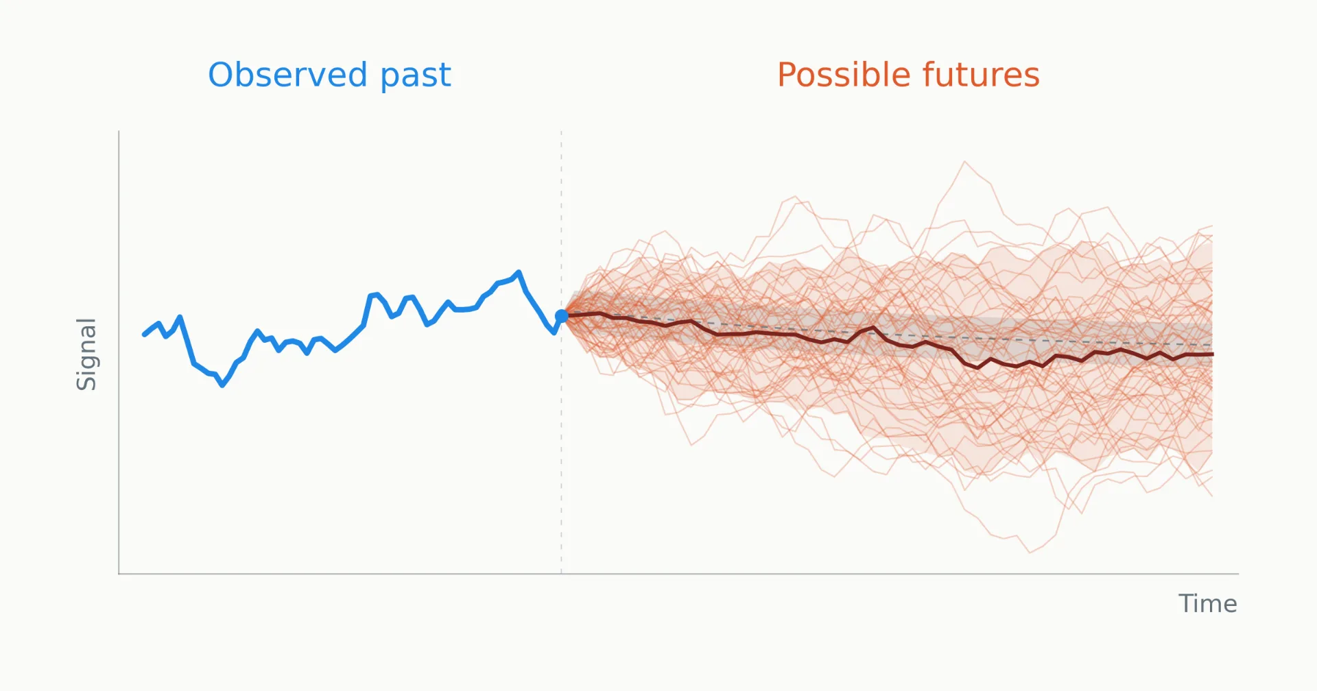
Read the full article at Towardsdatascience →KhanList aggregates and links to publicly available news content. We do not host full articles from third-party sources. Always verify important information with original sources.