
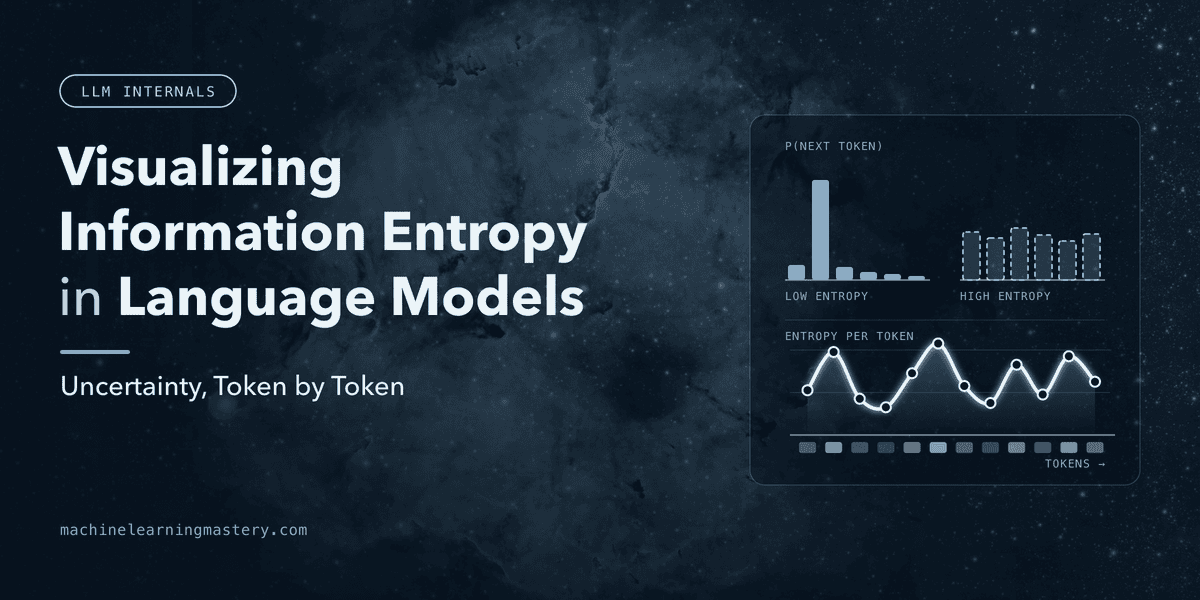
In this article, you will learn how information entropy and cross-entropy loss connect classical information theory to the way large language models are trained to predict the next word. Topics we will cover include: What information entropy measures, illustrated with a fair die and a weighted one. How cross-entropy loss compares a model’s predicted next-word distribution with the true one during training. How to compute and visualize entropy and cross-entropy for three example model predictions in Python with Plotly. Introduction Ever trained a neural network for classifying images or read a recent paper about large language models (LLMs)? If so, chances are you came across a somewhat intimidating term: cross-entropy loss. Did you know this is the guiding compass for training (via optimization) massive models used on a daily basis, including Gemini, Llama, and GPT? Indeed, yes! But one question might pop into mind: why “entropy”? Perhaps you might have seen that term in a different context, like information theory. Let’s bridge the gap between these pieces and better understand how entropy and information theory principles are leveraged to teach modern AI systems to “speak”. Once we link these concepts together, we’ll perform a Python-based visualization to better understand how information entropy is used in LLMs. Information Entropy Demystified Let’s trace back to 1948, the year classical information theory was born. Specifically, the concept of information entropy, or simply entropy, was introduced by Claude Shannon as a mathematical measure of uncertainty or “surprise” in a probability distribution. Take two dice as an example: let die A be totally fair, with every roll being unpredictable. When rolling this die, uncertainty is at its maximum, which means entropy would be quantified as high. Meanwhile, suppose die B is strongly weighted to land on its 6 face. You’d rarely be surprised by the outcome, as you’d expect a 6 most of the time: this is a low-uncertainty, low-entropy scenario. In other words, die B’s probability distribution is far from uniform, with a result of 6 being much more probable than the others. Mathematically, the entropy $H$ for a probability distribution $P$ can be calculated as: $$H(P) = – \sum P(x) \log_2 P(x)$$ This formula yields maximum entropy when all probabilities are equal (a uniform distribution, just like die A). Conversely, the more the probability of some outcomes stands out from the rest, the lower the entropy and uncertainty. Bringing Information Entropy into LLMs: Cross-Entropy Loss At their top layer, just before generating final outputs — words or tokens in a response — LLMs act as “uncertainty engines”. They don’t generate a whole text in one shot but iteratively play the game of “guessing the next word”. Imagine the model has so far generated the sequence: “the cat sat on the …”. The LLM’s top layer considers the model’s entire vocabulary, typically tens of thousands of words, assigning probabilities to every possible word. These are the possible scenarios at this point: When the model is uncertain about the next (most probable) word to generate, the probability distribution over this vocabulary would look spread out, close to uniform, thus being in a high-entropy state. If the model is highly confident about a specific word, for instance “tatami”, it assigns a very high probability to that word, and near-zero to everything else: that’s a low-entropy state. When an LLM is trained, the natural aim to pursue is minimizing its uncertainty about the correct next word, gradually having the model become more and more confident about its capabilities to generate text outputs word by word. So, what is cross-entropy loss? It is a loss function used to guide the training process, namely seeking to minimize it as much as possible. It measures the difference between two probability distributions: the true distribution reflecting what actually happened and the predicted distribution, i.e. what the model guesses. To better understand this, imagine the true next word in a training example is “tatami”. The ground-truth distribution acts just like the known labels in classical machine learning models, and it is equal to a probability of 100% for “tatami” and 0% for the rest of the words in the vocabulary. Thus, cross-entropy measures how far the next-word probability distribution calculated by the model for the training example “the cat sat on the…” is from the one-hot, ground-truth distribution. Telling the model to minimize cross-entropy during training is equivalent to forcing it to gradually shift its confidence toward correct words. When this is done over millions or billions of different training examples during many iterations, we eventually get our LLM to learn to generate responses that make sense! Let’s visualize and put all these ideas together through a code-based example that you can easily run in a notebook or Python script. This is a very lightweight script that doesn’t load an actual LLM, but closely illustrates how the concept of cross-entropy works inside the top layer of these models. We set up a small vocabulary with just five possible words to choose from, and assume the true next word or target associated with a training example would be “cat”. The true distribution with respect to the vocabulary is stored in a variable named P: this is one of the two inputs for calculating cross-entropy. For the second input, we consider three different scenarios — for instance, the outputs of three different LLMs with different levels of confidence or certainty. We store these three cases in a Python dictionary named models: 1234567891011121314151617 import numpy as npimport plotly.graph_objects as gofrom plotly.subplots import make_subplots# 1. Setup: A tiny vocabularyvocab = ["apple", "banana", "cat", "dog", "elephant"]target_word = "cat"# TRUE distribution (Target token is "cat", index 2)P = np.array([0.0, 0.0, 1.0, 0.0, 0.0])# 2. Three Model Predictions: suppose they have been computed by an LLM's final layermodels = { "Confident & Correct": np.array([0.02, 0.03, 0.90, 0.03, 0.02]), "Confident & Wrong": np.array([0.80, 0.05, 0.05, 0.05, 0.05]), "Uncertain (Flat)": np.array([0.20, 0.20, 0.20, 0.20, 0.20]),} All it takes now is to calculate the cross-entropy between the true distribution and each of the three “model” distributions. We also use plotly to visualize these three distributions in interactive bar plots, using this code: 12345678910111213141516171819202122232425262728293031323334353637383940414243444546474849505152535455565758 # 3. Math Functionsdef shannon_entropy(dist): """Measures internal uncertainty in bits.""" return -np.sum(dist * np.log2(dist + 1e-9))def cross_entropy(true_dist, pred_dist): """Measures loss against true target.""" return -np.sum(true_dist * np.log2(pred_dist + 1e-9))# 4. Build Interactive Subplotssubplot_titles = [ f"{name}Entropy: {shannon_entropy(q):.2f} bits | Loss: {cross_entropy(P, q):.2f}" for name, q in models.items()]fig = make_subplots( rows=1, cols=3, subplot_titles=subplot_titles, shared_yaxes=True)for col_idx, (name, Q) in enumerate(models.items(), start=1): # Color target token green ('cat') and distractors blue colors = ['#2ca02c' if word == target_word else '#1f77b4' for word in vocab] # Custom hover cards hover_labels = [ f"Token: {word}" f"Probability: {prob:.1%}" f"Target Token: {'Yes' if word == target_word else 'No'}" for word, prob in zip(vocab, Q) ] fig.add_trace( go.Bar( x=vocab, y=Q, marker_color=colors, hoverinfo="text", hovertext=hover_labels, name=name, showlegend=False ), row=1, col=col_idx )# 5. Styling Layoutfig.update_layout( title_text="Language Model Predictions: Entropy vs. Cross-Entropy Loss", title_x=0.5, yaxis_title="Probability", yaxis=dict(range=[0, 1]), template="plotly_white", height=450, margin=dict(t=100, b=40, l=60, r=40))fig.show() Resulting visualization: Which model would you choose by looking at these results? While both standalone information entropy and cross-entropy clearly point to the first model, the interesting question here is: which one is the worst? Information entropy is at its maximum in the right-hand model, which is completely uncertain about the choice to make. However, while the middle model is confident in choosing “apple”, it made an incorrect prediction, as correctly captured by an unacceptably high value for its cross-entropy. Both cases (high uncertainty and incorrect predictions) are simultaneously tackled by trying to reduce a model’s cross-entropy during training. Wrapping Up This article bridged the gap between the theory of information entropy and modern LLMs, highlighting how the latter make use of the former in their underlying components to generate text outputs effectively. The discussion was accompanied by a code example you can try yourself to visualize several examples of cross-entropy calculation. No comments yet.
Visualizing Information Entropy in Language Models
Full Article
Original Source
Read the full article at Machinelearningmastery →KhanList aggregates and links to publicly available news content. We do not host full articles from third-party sources. Always verify important information with original sources.