# Introduction Time series feature engineering doesn't follow the same rules as tabular data. Observations aren't independent, row order isn't incidental, and the most useful features are rarely individual readings. You'll have to identify patterns across time like rates of change, lag comparisons, deviations from a rolling baseline, and more. Building lags, sliding windows, and grouping across resolutions are all, at their core, iteration problems over ordered sequences. Python's itertools module is a natural fit for this kind of work. It doesn't replace high-level pandas abstractions like .rolling(), but it gives you lower-level building blocks to construct exactly the features you need, with full control over the logic. In this article, you'll build seven categories of time series features using itertools. You'll also apply each to a sample dataset. You can get the code on GitHub. # Creating a Sample Dataset Before we start building the features, let's spin up a sample sensor dataset to work with throughout the article. import numpy as np import pandas as pd import itertools np.random.seed(42) periods = 168 # one week of hourly readings index = pd.date_range(start="2024-03-01", periods=periods, freq="h") hours = np.arange(periods) # Temperature (°C): daily cycle + gradual drift + noise temp_base = 3.5 temp_daily = 1.2 * np.sin(2 * np.pi * hours / 24) temp_drift = 0.003 * hours temp_noise = np.random.normal(0, 0.3, periods) temperature = temp_base + temp_daily + temp_drift + temp_noise # Humidity (%): inverse relationship with temperature + noise humidity = 78 - 2.1 * (temperature - temp_base) + np.random.normal(0, 1.2, periods) # Power draw (kW): peaks during business hours, higher on weekdays day_of_week = index.dayofweek business_hours = ((index.hour >= 8) & (index.hour = 5, 0.6, 1.0) power = ( 42.0 + 18.0 * business_hours * weekend_factor + np.random.normal(0, 2.1, periods) ) df = pd.DataFrame({ "temperature_c": np.round(temperature, 3), "humidity_pct": np.round(humidity, 2), "power_kw": np.round(power, 2), }, index=index) df.index.name = "timestamp" print(df.head(8)) print(f"\nShape: {df.shape}") Output: temperature_c humidity_pct power_kw timestamp 2024-03-01 00:00:00 3.649 77.39 40.27 2024-03-01 01:00:00 3.772 76.52 41.33 2024-03-01 02:00:00 4.300 75.25 42.87 2024-03-01 03:00:00 4.814 74.26 40.82 2024-03-01 04:00:00 4.481 75.85 40.27 2024-03-01 05:00:00 4.604 76.09 42.51 2024-03-01 06:00:00 5.192 74.78 42.51 2024-03-01 07:00:00 4.910 76.03 40.94 Shape: (168, 3) We now have 168 hourly readings across three sensor channels. Now let's build features. # 1. Generating Lag Features with islice Lag features are the most fundamental time series feature: the value of a variable at a fixed number of steps in the past. For example, values from 1 step ago, 6 steps ago, or 24 steps ago can each capture distinct patterns such as short-term fluctuations, recurring intra-period behavior, and longer-term trends or seasonality. Let's build lag features for our sample dataset using islice: sensor_readings = df["temperature_c"].tolist() lag_offsets = [1, 6, 12, 24] lag_features = {} for lag in lag_offsets: lagged = list(itertools.islice(sensor_readings, 0, len(sensor_readings) - lag)) # Pad the beginning with None to preserve index alignment lag_features[f"temp_lag_{lag}h"] = [None] * lag + lagged lag_df = pd.DataFrame(lag_features, index=df.index) lag_df["temperature_c"] = df["temperature_c"] print(lag_df.iloc[24:30]) Output: temp_lag_1h temp_lag_6h temp_lag_12h temp_lag_24h \ timestamp 2024-03-02 00:00:00 2.831 2.082 3.609 3.649 2024-03-02 01:00:00 3.409 1.974 2.654 3.772 2024-03-02 02:00:00 3.919 2.960 2.425 4.300 2024-03-02 03:00:00 3.833 2.647 2.528 4.814 2024-03-02 04:00:00 4.542 2.986 2.205 4.481 2024-03-02 05:00:00 4.443 2.831 2.486 4.604 temperature_c timestamp 2024-03-02 00:00:00 3.409 2024-03-02 01:00:00 3.919 2024-03-02 02:00:00 3.833 2024-03-02 03:00:00 4.542 2024-03-02 04:00:00 4.443 2024-03-02 05:00:00 4.659 islice(sensor_readings, 0, len - lag) extracts the sequence shifted back by lag steps without creating a copy of the full list. The None padding at the front keeps every lag feature aligned with the original index. This matters when you later drop NaNs for model training. # 2. Building Rolling Window Features with islice and accumulate A single lag value tells you what the sensor read at a point in the past. A rolling statistic tells you what the sensor has been doing over a window of time, which is often far more useful. readings = df["temperature_c"].tolist() window_size = 6 # 6-hour rolling window rolling_features = [] for i in range(len(readings)): if i 0 and std_b > 0 else None correlations.append(corr) pairwise_features[feature_name] = correlations corr_df = pd.DataFrame(pairwise_features, index=df.index) print(corr_df.iloc[12:18]) Output: corr_temp_humi_12h corr_temp_powe_12h \ timestamp 2024-03-01 12:00:00 -0.6700 -0.2281 2024-03-01 13:00:00 -0.7208 -0.4960 2024-03-01 14:00:00 -0.7442 -0.6669 2024-03-01 15:00:00 -0.7678 -0.7076 2024-03-01 16:00:00 -0.8116 -0.7265 2024-03-01 17:00:00 -0.8368 -0.7482 corr_humi_powe_12h timestamp 2024-03-01 12:00:00 0.5380 2024-03-01 13:00:00 0.6614 2024-03-01 14:00:00 0.7202 2024-03-01 15:00:00 0.7311 2024-03-01 16:00:00 0.7233 2024-03-01 17:00:00 0.7219 # 7. Accumulating Running Baselines with accumulate A given value can carry different significance depending on when it occurs in a sequence. What matters is its deviation from the evolving baseline — the running mean up to that point in time. Using an incremental approach such as accumulate, you can compute this running mean efficiently without storing the entire history. readings = df["temperature_c"].tolist() running_sums = list(itertools.accumulate(readings)) running_counts = list(itertools.accumulate([1] * len(readings))) running_means = [ round(s / c, 4) for s, c in zip(running_sums, running_counts) ] # Running max — highest temperature seen so far, useful for breach tracking running_max = list(itertools.accumulate(readings, func=max)) deviation_from_baseline = [ round(r - m, 4) for r, m in zip(readings, running_means) ] baseline_df = pd.DataFrame({ "temperature_c": readings, "running_mean": running_means, "running_max": running_max, "deviation_from_baseline": deviation_from_baseline, }, index=df.index) print(baseline_df.iloc[20:28]) Output: temperature_c running_mean running_max \ timestamp 2024-03-01 20:00:00 2.960 3.5857 5.192 2024-03-01 21:00:00 2.647 3.5430 5.192 2024-03-01 22:00:00 2.986 3.5188 5.192 2024-03-01 23:00:00 2.831 3.4902 5.192 2024-03-02 00:00:00 3.409 3.4869 5.192 2024-03-02 01:00:00 3.919 3.5035 5.192 2024-03-02 02:00:00 3.833 3.5157 5.192 2024-03-02 03:00:00 4.542 3.5524 5.192 deviation_from_baseline timestamp 2024-03-01 20:00:00 -0.6257 2024-03-01 21:00:00 -0.8960 2024-03-01 22:00:00 -0.5328 2024-03-01 23:00:00 -0.6592 2024-03-02 00:00:00 -0.0779 2024-03-02 01:00:00 0.4155 2024-03-02 02:00:00 0.3173 2024-03-02 03:00:00 0.9896 # Summary Time series feature engineering is fundamentally about describing context — what has this signal been doing, relative to what we expect it to be doing? Every function covered here is a different way of formalizing that question into a number a model can learn from. Here's a summary of the patterns we've covered in this article: itertools Function Time Series Feature Example islice Lag features Temperature 1h, 6h, 24h ago islice + accumulate Rolling window stats 6h mean, std, min, max product Seasonal interaction grid Hour × day type × shift baseline tee Parallel window statistics Mean + range + rate of change chain Multi-resolution feature assembly Raw + rolling + calendar features combinations Pairwise cross-sensor correlations Temp–humidity, temp–power rolling corr accumulate Running baseline + deviation Drift detection from historical mean And because itertools works at the iterator level, all of these patterns compose cleanly into streaming pipelines as well. Happy feature engineering! Bala Priya C is a developer and technical writer from India. She likes working at the intersection of math, programming, data science, and content creation. Her areas of interest and expertise include DevOps, data science, and natural language processing. She enjoys reading, writing, coding, and coffee! Currently, she's working on learning and sharing her knowledge with the developer community by authoring tutorials, how-to guides, opinion pieces, and more. Bala also creates engaging resource overviews and coding tutorials.
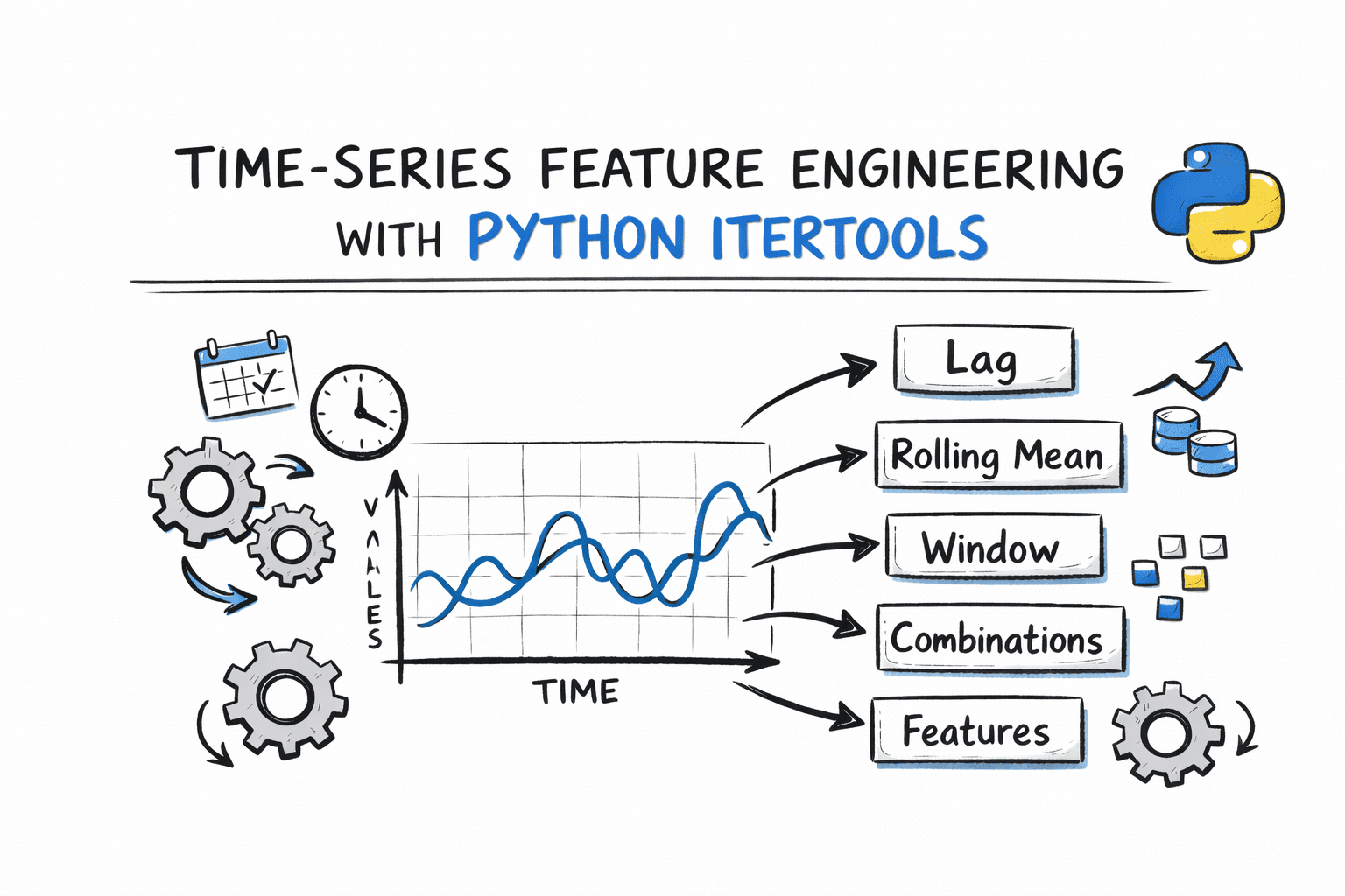
Time-Series Feature Engineering with Python Itertools
Full Article
Original Source
Read the full article at Kdnuggets →KhanList aggregates and links to publicly available news content. We do not host full articles from third-party sources. Always verify important information with original sources.