Stop Calling the First Significant Day a Win

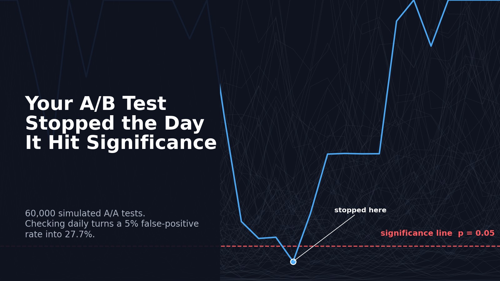
in a fairly straightforward way. They launch a test, open the dashboard every morning, and wait for the p-value to drop below 0.05. When it does, the result looks official enough to ship. The line has been crossed, the number looks clean, and the winner seems ready to call. I would not say that this routine is always done carelessly. In most cases, the team is doing exactly what the standard tutorial taught them to do: define the hypothesis, pick the metric, run the two-proportion z test or t test, and reject the null when p falls below 0.05. Some guides even add the valuable step of calculating the required sample size before the test starts. But there is one crucial thing that often gets missed. The 5 percent false-positive rate is written for one look at one fixed sample, and the math changes once the same dashboard is checked again and again before the experiment ends. I ran a simulation to make this visible. The setup was deliberately ordinary: two versions, A and B, both converting at the same true 10 percent rate; 1,000 visitors per arm per day; a two-sided test at the 5 percent level; and 30 days of traffic. Nothing was different between A and B. There was no product improvement to find. The only thing the test could discover was noise. import numpy as np from scipy import stats RNG = np.random.default_rng(5) n_sims = 60_000 n_days = 30 visitors_per_arm_day = 1_000 p_true = 0.10 def two_prop_z(succ_a, n_a, succ_b, n_b): pa, pb = succ_a / n_a, succ_b / n_b pool = (succ_a + succ_b) / (n_a + n_b) se = np.sqrt(pool * (1 - pool) * (1 / n_a + 1 / n_b)) z = (pb - pa) / se return z, 2 * stats.norm.sf(np.abs(z)) inc_a = RNG.binomial(visitors_per_arm_day, p_true, size=(n_sims, n_days)) inc_b = RNG.binomial(visitors_per_arm_day, p_true, size=(n_sims, n_days)) cum_a, cum_b = inc_a.cumsum(axis=1), inc_b.cumsum(axis=1) n = np.cumsum(np.full((n_sims, n_days), visitors_per_arm_day), axis=1) _, p_daily = two_prop_z(cum_a, n, cum_b, n) false_positive_daily = (p_daily boundary).any(axis=1).mean() # In the seeded run used here, the calibrated constant boundary is 2.73, # compared with the usual fixed-sample 1.96. pocock_boundary = 2.73 fp_pocock = false_positive_at_boundary(z_daily, pocock_boundary) # Always-valid p-value from a mixture sequential probability ratio test TAU = 0.01 # prior SD on the true absolute difference, about 1pp on a 10% base def msprt_pvalue(diff, var): tau2 = TAU ** 2 lam = np.sqrt(var / (var + tau2)) * np.exp( diff**2 * tau2 / (2 * var * (var + tau2)) ) return np.minimum(1.0, 1.0 / lam) MethodFalse-positive rate under the nullPower vs true 10% liftTypical days to decideFixed sample, no peeking5.1%97.9%30Daily peeking, naive 0.0527.7%not meaningfulabout 5Daily peeking, Pocock boundary4.9%93.3%11Daily peeking, always-valid p-value1.5%87.5%14 This is the part that is often missed in product discussions. The corrected methods make the result more honest while keeping much of the speed that made peeking attractive in the first place. Speed only becomes a problem when it sits outside the design. Against a true 10 percent lift, the fixed-sample design caught the effect 97.9 percent of the time, but only at day 30 by design. The Pocock boundary caught it 93.3 percent of the time with a typical decision by day 11. The always-valid p-value caught it 87.5 percent of the time with a typical decision by day 14. That is the useful tradeoff. You can stop early when the effect is real, but you are no longer pretending that the first naive p < 0.05 means the same thing as a single fixed-sample test. The speed becomes part of the design instead of an informal habit layered on top of it. The always-valid method is more conservative in this setup, because it is paying for a guarantee that holds at any stopping time. The prior used in the simulation can also be tuned. If a team sets it closer to the effect size it genuinely expects, it can recover power. The choice of method depends on how the team wants to run the experiment, but the method has to know the team is looking. A few limits worth saying out loud This simulation measures one slice of the problem: one metric, one treatment against one control, clean randomization, and steady daily traffic. Real experimentation programs are usually messier. Teams test multiple metrics, several variants, and sometimes several segments at the same time. Each of those choices adds another layer of multiplicity, so the numbers here are closer to a floor than a worst case. The simulation also does not solve novelty effects or weekday patterns. If users react differently in the first few days because something is new, or if the business has strong day-of-week cycles, a minimum runtime of one or two full weeks may still be necessary regardless of the sequential method. Variance-reduction methods such as CUPED are also complementary. They reduce the sample size needed, but they do not by themselves fix the stopping-rule problem. So the practical lesson is not to stop looking at the dashboard. Teams will look at the dashboard, and that is fine. The act of looking just has to be part of the design, not something that happens outside the statistics. What the next A/B testing guide should teach A better A/B testing guide would make four changes. First, state the stopping rule before the test starts, the same way you state the metric and the hypothesis. The stopping rule determines whether the p-value will mean anything when you use it. Second, if you will look once, do the power calculation and commit to the sample size. This is the highest-value basic habit and it is already available to anyone who can compute an effect size. Third, if you will look repeatedly, use a method built for repeated looks. A group-sequential boundary works when the number of looks is fixed in advance. An always-valid p-value works when the team wants the freedom to check whenever it wants. Fourth, report the stopping rule next to the result. A reader should be able to see whether the 5 percent claim is real, or whether it only looks real because the test stopped on the lucky day. The z test is sound when it is used in the setting it was built for. The error comes from using a guarantee written for one fixed look to justify repeated looks. Choose a stopping rule that matches how the team actually behaves, and the p-value can keep the meaning it was supposed to have. References Armitage, P., McPherson, C. K., and Rowe, B. C. Repeated Significance Tests on Accumulating Data. Journal of the Royal Statistical Society Series A, 1969. Wald, A. Sequential Analysis. Wiley, 1947. Pocock, S. J. Group Sequential Methods in the Design and Analysis of Clinical Trials. Biometrika, 1977. O’Brien, P. C., and Fleming, T. R. A Multiple Testing Procedure for Clinical Trials. Biometrics, 1979. Lan, K. K. G., and DeMets, D. L. Discrete Sequential Boundaries for Clinical Trials. Biometrika, 1983. Johari, R., Koomen, P., Pekelis, L., and Walsh, D. Always Valid Inference: Continuous Monitoring of A/B Tests. Operations Research, 2022. Howard, S. R., Ramdas, A., McAuliffe, J., and Sekhon, J. Time-uniform, Nonparametric, Nonasymptotic Confidence Sequences. Annals of Statistics, 2021. Deng, A., Lu, J., and Chen, S. Continuous Monitoring of A/B Tests without Pain: Optional Stopping in Bayesian Testing. IEEE DSAA, 2016. Kohavi, R., Tang, D., and Xu, Y. Trustworthy Online Controlled Experiments. Cambridge University Press, 2020. Simmons, J. P., Nelson, L. D., and Simonsohn, U. False-Positive Psychology. Psychological Science, 2011. Reproducibility note: the figures and rates in this article come from a seeded Python simulation using numpy, scipy, and matplotlib. No external dataset is used. Each experiment is simulated from known ground truth, which is the only way to measure a false-positive rate directly. The key simulation and method-calibration code is included above; the reported rates are Monte Carlo estimates from the seeded run and can vary by a few tenths of a percentage point across seeds.