Reducing Human Annotation with ML Active Learning

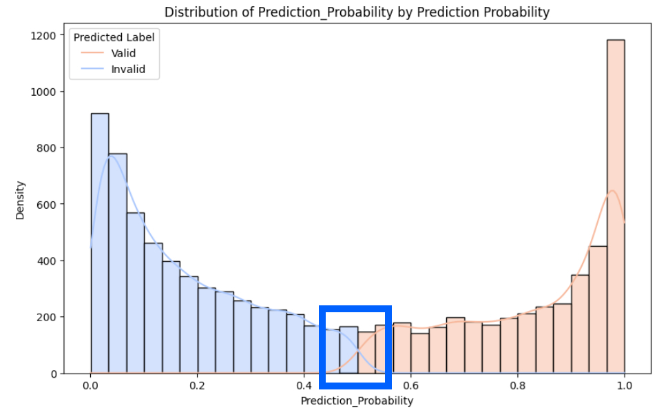
Active learning aims to select the unlabeled samples that are most informative and ask for labels only for those samples. By interactively querying a user (or some other information source) to label new data points, we can train models using less labels. This tutorial/tutorial walks you through the active learning workflow and shows you how to implement three commonly used query strategies: uncertainty sampling, diversity based sampling and query by committee. We provide intuitive explanations of these methods along with Python implementations. Finally, we will discuss the pros and cons of each method and how they can be used together to create powerful human-in-the-loop systems when annotation is expensive/scarcely available. of Contents What is Active Learning Learning from Uncertain or Edge-Case Samples Active Learning Techniques Uncertainty Sampling Diversity-based Sampling Query By Committee (QBC) Pros and Cons of Active Learning Benefits of Active Learning Limitations of Active Learning How to Choose the Right Strategy in Practice Conclusion 1. What Is Active Learning Active learning is an approach to machine learning in which a learning algorithm is able to interactively query a user (or some other information source) to obtain the desired outputs at new data points. In active learning, rather than feeding a learning algorithm a massive pool of labeled examples, you allow the model to look at the unlabeled data points first. It will pick the data points it wants to learn from and send only those to the human for labeling. You repeat this process in cycles. Using active learning, you can often achieve comparable performance to normal supervised learning with many fewer annotated training examples. See figure 1 for the active learning cycle. Figure 1. Diagram of the active learning iterative process (source: doi.org/10.1109/ACCESS.2025.3624650) Particularly when humans are in the loop, this technique shines. Rather than having the annotator label thousands of simple/redundant samples, the model instead surfaces which examples it’s least certain about or which examples appear odd/outlier, and then have the annotator label those. To understand the significance of Active Learning, think about an image classification task with 500,000 images. At 20 seconds per image, it will take over 2,700 hours to label this dataset. With active learning, you only request human attention to a few of these images that actually need help to improve your model substantially. This drastically cuts costs and the effort needed to label. 1.1. Learning From Uncertain or Edge-Case Samples One major benefit of active learning is that your model can focus on learning from the most difficult examples. Typically these examples fall around the decision boundary where your model is most uncertain and have the largest potential to improve the model. Effectively this allows your dataset to be enriched with targeted samples. The dataset size will not increase with synthetic transformations, but it will gain valuable information with the addition of new samples. Imagine training a model for self-driving cars. There are some rare events that may not be present frequently enough to be captured while collecting raw data. A cyclist coming out from behind a parked car is a great example. With active learning these rare cases can be presented early on and delivered to human annotators for review. The same could be said for a fraud detection model where you may want your model to direct human reviewers to suspicious activity versus transactions that are clearly legitimate or clearly fraud. If you’d like to follow along with the code for each step you can run and download the companion notebook here: https://github. com/lucasbraga461/active-learning/blob/main/active-learning/notebook.ipynb If you’d like to learn more about the theory behind this implementation, you can access my research paper here, it’s free access: https://doi.org/10.1109/ACCESS.2025.3624650 2. Active Learning Techniques The intuition behind active learning is using a query strategy to determine which unlabeled samples should be labeled first. Rather than randomly picking samples from our pool, we query the model about what samples it would like to look at. Typically these are samples that will help the model make better predictions. Active learning tends to be useful when labels are slow to acquire, require expert knowledge, or are costly. There are many strategies that generally trade-off exploration and exploitation of the regions where the model has the largest uncertainties. These methods have been applied in vision-based tasks, document classification, anomaly detection, and even medicine. Below we’ll go over three of the most common query strategies in an intuitive manner: uncertainty sampling, diversity-based sampling, query by committee. Dataset note: The examples in this article use a synthetic dataset created only for demonstration purposes. 2.1. Uncertainty Sampling Uncertainty sampling is often the first approach practitioners attempt because it requires very little effort and often leads to good initial gains. Uncertainty sampling is conceptually simple. You start off by labeling only enough samples to create your initial training set. Train your initial model on these samples. This initial model doesn’t have to be great! All we need it to do is make rough estimates of the probabilities for our unlabeled samples. Once we’ve trained the model, we identify the samples about which the model is least certain. These are usually the ones for which it predicts probabilities close to the decision threshold. Then we have these uncertain samples labeled by a human and retrain our model on this new data! If we repeat this process, our model incrementally improves upon its understanding where it’s least confident. You should see quicker gains then if you labeled many easy/redundant examples. 2.1.1. Train the First Model With Cross-Validation Before querying uncertain samples, we first need a model that performs reasonably well even when there is not much labeled data available. An easy way to accomplish this is to split the labeled data into training and validation folds, then run a small hyperparameter search using cross-validation to prevent overfitting. The result of splitting the dataset in Code Block 1 can be seen in Figure 2. Code Block 1. Split X and y X = df_i1.drop(columns=['label']) y = df_i1['label'] X Figure 2. Visualization of the dataframe independent features (X) Teams usually run lighter grid searches with 3 or 5 folds in practice, so don’t feel that you need this many folds when applying this process to your projects. Code Block 2. Train a model using nested cross-validation. # Hyperparameter grid and CV settings param_grid = {"C": [0.001, 0.01, 0.1, 1, 10, 100]} inner_cv = StratifiedKFold(n_splits=5, shuffle=True, random_state=42) outer_cv = StratifiedKFold(n_splits=5, shuffle=True, random_state=7) fold_metrics = [] best_params_each_fold = [] for train_idx, test_idx in outer_cv.split(X, y): X_train, X_test = X.iloc[train_idx], X.iloc[test_idx] y_train, y_test = y.iloc[train_idx], y.iloc[test_idx] grid = GridSearchCV( LogisticRegression(max_iter=500), param_grid, cv=inner_cv, scoring="f1", n_jobs=-1 ) grid.fit(X_train, y_train) best_model = grid.best_estimator_ best_params_each_fold.append(grid.best_params_) preds = best_model.predict(X_test) fold_metrics.append({ "precision": precision_score(y_test, preds), "recall": recall_score(y_test, preds), "f1": f1_score(y_test, preds) }) # Use the most frequent best parameters to train the final model final_params = pd.DataFrame(best_params_each_fold).mode().iloc[0].to_dict() final_model = LogisticRegression(**final_params, max_iter=500) final_model.fit(X, y) Now that we have our cross validated model we can apply it to our unlabeled set to get a measure of uncertainty. Figure 3 below shows what dataset fold_metrics looks like from Code Block 2. Figure 3. Cross Validation results and best parameters 2.1.2. Score the Unlabeled Data and Inspect the Probabilities We now want to calculate predicted probabilities for every sample in our unlabeled pool. Plotting these scores can help us see where our model is least confident. Code Block 3. Visualize the distribution of the predicted scores import seaborn as sns def plot_prediction_distribution(df, column_name): if column_name not in df.columns: raise ValueError(f"Column '{column_name}' not found in dataframe.") if "Prediction_Probability" not in df.columns: raise ValueError("Column 'Prediction_Probability' not found in dataframe. Ensure predictions were added.") # Ensure Predicted_Label is correctly assigned (1 = Valid, 0 = Invalid) plt.figure(figsize=(10, 6)) sns.histplot(df, x=column_name, hue="Predicted_Label", bins=30, kde=True, palette="coolwarm") plt.title(f"Distribution of {column_name} by Prediction Probability") plt.xlabel(column_name) plt.ylabel("Density") # Corrected Legend Order (1 = Valid, 0 = Invalid) plt.legend(title="Predicted Label", labels=["Valid", "Invalid"]) plt.show() from helpers import prediction_plots # Get probability scores new_probabilities = final_model.predict_proba(X_unlabeled)[:, 1] X_unlabeled["Prediction_Probability"] = new_probabilities prediction_plots.plot_prediction_distribution(X_unlabeled, "Prediction_Probability") Because this is a binary classification problem our model will often be least certain with probabilities near 0.5. This represents where AL can be the most valuable. Figure 4 below is what the plot looks like from running Code Block 3. Figure 4. Distribution of the scores from the first iteration on unlabeled data 2.1.3. Choose Samples Inside the Uncertainty Window For our next batch to label we will focus on an area around the decision threshold. We can define a small band around 0.5 then sample from that region. Figure 5 below displays the resulting plot from running Code Block 4. center = 0.50 lower = center - 0.05 upper = center + 0.05 mask = (X_unlabeled["Prediction_Probability"] > lower) & \ (X_unlabeled["Prediction_Probability"] <= upper) batch_size = 60 selected_batch = X_unlabeled[mask].sample(batch_size, random_state=42) Figure 5. Unlabeled dataset with prediction probability from the first iteration These samples should represent where our model is least confident. 2.1.4. Iterate Now repeat the cycle: Train the model Predict probs on unlabeled set Select samples closest to uncertain region Label those and Rinse and repeat As this cycle continues the model should become more confident and the uncertain region will become smaller. When this process starts to plateau you can add in more exploratory techniques like diversity sampling or committee-based sampling. 2.1.5. Strengths and Weaknesses of Uncertainty Sampling Strenghts Easy to implement and low computational cost. Can use any model that outputs probability estimates. Extremely useful when labeling is costly or when you have limited amounts of data. Weaknesses May excessively focus on a small region of the feature space. Relies on model’s ability to accurately estimate probabilities. May select highly similar edge cases over and over again without exploring the data-set as a whole. Summary: Uncertainty Sampling Most effective when used in the early iterations of modeling when the model has not quite defined the boundary. Ultra Efficient since it only requires model probability estimates. May focus too narrowly if used for too many iterations without other forms of exploration. 2.2. Diversity-Based Sampling Diversity-based sampling can be considered another extension of active learning where labeling choices are made based upon how diverse/uncommon each unlabeled sample is when compared to all other samples within the feature space. Instead of simply choosing where your model is most uncertain you attempt to choose examples that cover more ground. This can allow your model to label more expressive examples and gain better overall insight into the data it is working with. Diversity-based sampling can be beneficial if your model begins to converge and you find yourself repeatedly querying the same types of edge cases with uncertainty sampling. By sampling more sparsely you will build a more representative training set which can lead to greater gains in future iterations. 2.2.1. Practical Example Let’s say you’ve already ran through a few iterations of uncertainty sampling and already have a couple hundred labeled samples. You’re likely beginning to see a sharp drop off in return because you’re bound to keep querying similar samples. Now would be a good time to take a diversity based step. In order to do this, we will consider each sample in our pool unlabeled and try to estimate how many nearest neighbors it has. Samples that are located within very dense clusters will likely be very similar to samples you’ve already trained on. Alternatively, samples that have very few neighbors are samples that may exist in more sparsely populated regions. A quick and dirty way to approximate this is to use sklearn’s KNN algorithm and find the average distance to your nearest neighbors. Remember to scale your features before computing distances with Euclidean. Refer to Figure 6 for an illustration of KNN. Figure 6. Illustration of how KNN works. Code Block 5 demonstrates an example workflow. Figure 7 illustrates the resulting dataset most_diverse from Code Block 5. Code Block 5. Select samples using diverse sampling strategy from sklearn.neighbors import NearestNeighbors # Fit the KNN model on the features of the unlabeled data knn = NearestNeighbors(n_neighbors=k, metric="euclidean") knn.fit(X_unlabeled[feature_cols]) # Compute average neighbor distance as a proxy for sparsity distances, _ = knn.kneighbors(X_unlabeled[feature_cols]) X_unlabeled["Density"] = distances.mean(axis=1) # Select the most diverse samples most_diverse = X_unlabeled.nlargest(n_samples, "Density") most_diverse.head() Figure 7. Unlabeled dataset with Density values from KNN The selected points usually make up a batch of between 50 and 60 samples. You label them, add them to your ever-growing training set, and retrain your model. From this point, you can see how your model’s predictions evolve, plot the probability distribution once more, or determine whether another round of diversity selection is beneficial before proceeding with active learning via another query strategy. 2.2.2. Advantages and Disadvantages of Diversity Sampling Advantages helps you build a more representative training set by exploring regions of the data that were previously underrepresented. fewer redundant samples when compared to repeatedly querying by uncertainty only. Disadvantages harder to implement than “vanilla” uncertainty sampling. distance metrics, clustering methods, or visual diagnostics needed to intelligently select samples. Summary Diversity Sampling promotes exploration of regions in your data which are not covered by your training set. Lowers redundancy when compared to only using uncertainty for sample selection. Depends on distance metrics or clustering, so can be slightly more expensive. 2.3. Query By Committee (QBC) Query by Committee maintains a committee of models rather than a single model. The committee members are each trained on the currently labeled data. Since different models may rely on different learning algorithms, or have different internal defaults, they may give slightly different answers. We can use this. When the committee votes wildly among its members, we know we’ve found a difficult/ambiguous sample that would do well to be manually labeled. Essentially, we search for points where committee members disagree and query those points for labeling. That way, the AL loop will focus on those samples that are most likely to give the biggest bang for your modeling buck. 2.3.1. Training a Committee of Models For our committee we’ll want models that reason about the data differently. As such, let’s train three different kinds of models: a linear model, a tree-based model, and a kernel model. Below is a function that will train four models on the currently-labeled data. Code Block 6. Train a committee of models def train_qbc_committee(X_train, y_train): """ Trains a small committee of diverse models for QBC. Returns a dictionary of fitted models. """ models = { "Logistic Regression": LogisticRegression(C=0.1, max_iter=500), "Random Forest": RandomForestClassifier(n_estimators=50, max_depth=5, min_samples_leaf=5), "Extra Trees": ExtraTreesClassifier(n_estimators=50, max_depth=5, min_samples_leaf=5), "SVM": SVC(kernel="rbf", C=0.1, probability=True) } trained = {} for name, model in models.items(): print(f"Training {name}...") model.fit(X_train, y_train) trained[name] = model return trained X = df_i6.drop(columns=["label"]) y = df_i6["label"] X_train, X_test, y_train, y_test = train_test_split( X, y, test_size=0.3, stratify=y, random_state=42 ) committee = query_by_committee.train_qbc_committee(X_train, y_train) Once this code has been run, we have a group of models that we can ask for individual predictions/probability estimates to use in the next step of the pipeline. 2.3.2. Evaluating the Committee and Building a Stacked Model Each committee member will output a probability for the positive class. We can take all of those probabilities, for each item in our pool, and build a new feature set that we can trivially train a meta-model on top of. This process is called stacking. Since Logistic Regression is trivial to interpret, and works well with this small number of stacking inputs, we will use it for our stacking layer. Table 1. Model Performance after QBC ModelBest parametersF1-ScorePrecisionRecallLogisticRegression‘C’: 0.0010.76880.69750.8564RandomForestClassifier‘max_depth’: 7, ‘min_samples_leaf’: 4, ‘n_estimators’: 1000.87530.87180.8806ExtraTreesClassifier‘max_depth’: 7, ‘min_samples_leaf’: 6, ‘n_estimators’: 1000.87720.86190.8977SVM‘C’: 10.92580.96360.8936 Code Block 7 below shows how to create these stacked features. Figure 8 is the resulting dataset from running the code. Code Block 7. Create a train and test set using the scores of the models trained X_train_scores = query_by_committee.stacking_models(X_train, committee) X_test_scores = query_by_committee.stacking_models(X_test, committee) X_train_scores[[ "Logistic Regression_score", "Random Forest_score", "Extra Trees_score", "SVM_score" ]].head() Figure 8. Dataset with multiple model scores to be used as features for model stacking Training the stacking layer Code Block 8. Train different models on top of the scores of the previous models trained. models_stacking = query_by_committee.train_qbc_committee( X_train_scores[[ "Logistic Regression_score", "Random Forest_score", "Extra Trees_score", "SVM_score" ]], y_train, cv_folds=5 ) stacked_results = model_evaluation.evaluate_model( models_stacking["Logistic Regression"], X_test_scores[[ "Logistic Regression_score", "Random Forest_score", "Extra Trees_score", "SVM_score" ]], y_test, threshold=0.50 ) Why stacking helps After stacking has been performed, increases in overall performance are common. One model might have high accuracy in one region of the data and another might excel elsewhere. One tree might capture nonlinear regions and an SVM may have been able to classify difficult boundaries. By stacking these models, you both utilize each of their strengths and limit the weaknesses of each individual learner. Table 2. Model Performance including model stacking ModelBest parametersF1-ScorePrecisionRecallLogisticRegression‘C’: 0.0010.76880.69750.8564RandomForestClassifier‘max_depth’: 7, ‘min_samples_leaf’: 4, ‘n_estimators’: 1000.87530.87180.8806ExtraTreesClassifier‘max_depth’: 7, ‘min_samples_leaf’: 6, ‘n_estimators’: 1000.87720.86190.8977SVM‘C’: 10.92580.96360.8936Stacking the models using LogisticRegression‘C’: 0.10.93600.92230.9500 Comparing metrics before and after stacking usually show that your stacked model has higher recall with only a slight loss in precision. For many applications, this tradeoff is worthwhile if it means your model rarely misses positive samples. Taken together, stacking allows you to create a balanced, robust learner that profits from diversity in your committee and improves your active learning loop. 2.3.3. Selecting Samples Where the Committee Disagrees After you have trained your committee, you can begin to evaluate how much the models in your committee disagree on each unlabeled sample’s prediction. The reasoning behind this method is fairly straightforward. If several models that typically do not agree happen to make the same prediction for a sample, that sample is unlikely to contain much information. However, if the models do disagree, that indicates that the sample probably exists in a region that the committee finds uncertain or unclear. One way to measure this is to calculate the variance of the predicted probabilities between models in the committee. Higher variance indicates more disagreement, which by extension means those samples are likely very useful if annotated. Code Block 9 includes an example function for computing these disagreement scores. Code Block 9. Function to create the disagreement_scores column def select_qbc_samples(X_unlabeled, models): """ Computes prediction disagreement for each unlabeled point based on the probability outputs from all committee models. """ X_scores = X_unlabeled.copy() base_features = X_unlabeled.iloc[:, :models["Logistic Regression"].n_features_in_] preds_matrix = np.zeros((base_features.shape[0], len(models))) for i, (name, model) in enumerate(models.items()): score_column = f"{name}_score" X_scores[score_column] = model.predict_proba(base_features)[:, 1] preds_matrix[:, i] = X_scores[score_column] # Variance across committee predictions X_scores["disagreement_score"] = np.var(preds_matrix, axis=1) return X_scores Once you have created these disagreement scores, you can sort your unlabeled data by this metric and select the top samples for labeling, shown in Code Block 10 and Figure 9. Code Block 10. Select the samples with the largest disagreement_score value X_unlabeled = query_by_committee.select_qbc_samples(X_unlabeled, models) num_samples = 60 most_uncertain = X_unlabeled.nlargest(num_samples, "disagreement_score") most_uncertain.head() Notice that this final batch of points should contain the samples where your committee members strongly disagreed with each other. These points should cover the areas of the decision boundary that were causing the largest disagreements between your models. By identifying these samples and labeling them, your model will be able to improve on some of these boundary regions when it is retrained. Figure 9. Dataset after-QBC with the disagreement scores Query by Committee in a nutshell Uses model disagreement as a measure for identifying informative samples. Works best when different models learn different things from the data. Takes time and resources to train and maintain multiple models. 3. Pros and Cons of Active Learning Active learning can become a vital component of your machine learning workflow by allowing you to shift your annotation efforts away from everything to only what matters. Like any technology there are numerous advantages and some real-world constraints. The sections below outline each in brief so you can determine if active learning will suit your use case. 3.1. Benefits of Active Learning 3.1.1. Reduce Annotation Costs For most problems labeling data is one of the largest investments of time and money. Active learning alleviates this pain point by allowing you to focus your annotation efforts only on samples that provide the most new information to your model. Label only these points and your team can achieve robust model performance without having to allocate resources to annotate at scale. 3.1.2. Fewer Labels for High-Quality Models Active learning attempts to query labels for the most difficult/informative examples. This means that every new label you add to your training set provides more value than if it were randomly sampled. You should expect to see much faster gains in accuracy/recall/F1 with an active learning framework, even with a small labeled dataset. 3.1.3. Ideal If Labeled Data Is Limited Companies and research teams are often faced with problems where labeled data will always be limited. Active learning allows you to create a framework for iteratively expanding that labeled dataset. It’s used commonly in any machine learning system that deals with perception, recommendations, anomaly detection, or other user-generated signals. 3.1.4. Works With Any ML Problem There is no one model or type of data that active learning has worked with. Customers have used it for fraud detection, NLP problems, image classification, time-series modeling, and more. If you’re looking for a way to leverage unlabeled data that would otherwise go to waste consider using active learning. 3.2. Limitations of Active Learning 3.2.1. Sampling Strategy Is Crucial Active learning is only as good as the samples you use to train your model. If your sampling strategy consistently returns noisy, deceptive, or uninformative samples your model may never converge. There is significant domain expertise required to pick an appropriate strategy. Once chosen, you’ll need to experiment to ensure that it works well in practice. 3.2.2. Sampling Bias Is Possible Uncertainty-based strategies tend to focus too intensely on smaller regions of your feature-space. Without intervention, your training-set will become unbalanced, limiting your ability to generalize. Uncertainty sampling should be paired with some sort of diversity checking to avoid this pitfall. 3.2.3. But we still need human experts One point to note about active learning is that although sample selection is automated, you still need humans in the loop to perform labeling. There are still some domains that are more dependent on human annotation like cybersecurity, clinical annotation, legal text review or certain vision tasks. 3.3. How to choose the right Strategy in Practice You can start with uncertainty sampling, specially if you have a small labeled dataset and/or you need early wins. Then add diversity sampling if you’ve taken already everything from uncertainty sampling and it’s started to not bring much better results. Use query by committee if decision boundaries are expected to be noisy OR you already have a committee of reasonable models you’d like to exploit. 4. Conclusion Active learning is straightforward in concept. Rather than labeling everything in your dataset, you label only the samples that your model needs to learn. When you’re operating in organizations where labeled samples are costly or time-consuming to produce, this difference has a significant impact. You’ll see your model improve at a faster rate, and your team only spends time labeling samples that have been vetted by your active learning loop. As with all design decisions, there are trade-offs. The loop introduces additional compute, and your results will change a lot based on your query strategy. Similarly prepared datasets will end-up with very different models if your query strategy produces redundant samples. Hence, it’s good practice to mix strategies. Uncertainty sampling works well at the start of a project to learn quickly, while diversity sampling helps you cover more of your feature space. Committee-based sampling allows you to focus on difficult-to-boundary samples. Combining them allows you to develop a more robust solution. Concluding, Active Learning helps you prioritize what samples to request human annotation, and it’s specially useful when you have many unlabeled samples and limited annotation resources. Image Note: All images in this article were created by the author unless otherwise stated.