I stopped using the Excel filter button to find high and low values. These 2 functions do it better

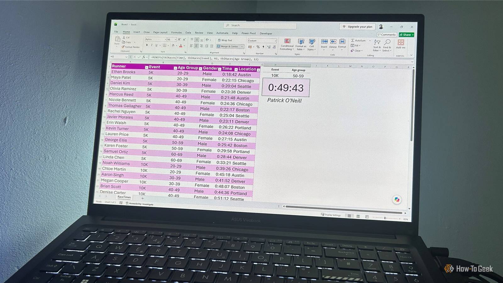
Published Oct 3, 2026, 7:00 AM EDT Tony Phillips is an experienced Microsoft Office user with a dual-honors degree in Linguistics and Hispanic Studies. Prior to starting with How-to Geek in January 2024, he worked as a document producer, data manager, and content creator for over ten years, and loves making spreadsheets and documents in his spare time. Tony is also an academic proofreader, experienced in reading, editing, and formatting over 3 million words of personal statements, resumes, reference letters, research proposals, and dissertations. Before joining How-To Geek, Tony formatted and wrote documents for legal firms, including contracts, Wills, and Powers of Attorney. Tony is obsessed with Microsoft Office! He will find any reason to create a spreadsheet, exploring ways to add complex formulas and discover new ways to make data tick. He also takes pride in producing Word documents that look the part. He has worked as a data manager in a secondary school in the UK and has years of experience in the classroom with Microsoft PowerPoint. He loves to encounter problems in Microsoft Office and use his expertise and legal-level training to find solutions. Outside of the Microsoft world, Tony is a keen dog owner and lover, football fan, astrophotographer, gardener, and golfer. Excel's filter button is useful, but I've realized I was relying on it for the wrong job. When all I wanted was the highest or lowest number that matched a certain condition, filtering meant hiding rows, sorting data, and then resetting everything afterward. But two functions I recently stumbled across have given me a much cleaner way to get those answers. Find high and low values without filtering your data Let Excel find the answer for you Credit: Lucas Gouveia/How-To Geek MAXIFS and MINIFS aren't just two more functions to add to your Excel toolbox. Since I learned about them, I've genuinely used them in several spreadsheets, and they've quietly become my go-to whenever I need to find the highest or lowest value that meets certain conditions. There's good reason for that. The old way of doing this is usually pretty simple: filter your data until you've got the records you want, sort the relevant column, and grab the number at the top or bottom. It works, but you're changing your view of the dataset just to answer a single question. If all I want is an answer, why rearrange my data to get it? MAXIFS and MINIFS leave everything where it is and return the answer in a cell. That means the result can sit in a summary table or dashboard, feed another formula, or power an Excel chart, while the underlying dataset remains fully visible. The formulas also update when the source data changes. If you add a new record, or an existing value changes, Excel recalculates the result without you having to remember which filters you applied or sort the data again. And then there's the biggest advantage: multiple criteria. You can ask Excel to find the highest or lowest value where several conditions are true at the same time. Instead of filtering one column, then another, and finally sorting what's left, you can describe the question in a single formula. MAXIFS finds the highest value that meets your criteria The syntax tells you almost everything you need to know The beauty of MAXIFS and its partner-in-crime is that their syntax makes them really easy to learn. The syntax for MAXIFS is: MAXIFS(max_range, criteria_range1, criteria1, [criteria_range2, criteria2], ...) In plain English, that means: find the highest value in one range, but only include values where the corresponding cells meet the specified criteria. So, for example, here's a table of computer specifications. Let's say I'm shopping for a new computer, and I've decided I don't want to spend more than $1,500. Before I start comparing individual models, I want to know how much RAM I can expect to get for that budget. I could filter the Price column to show computers costing $1,500 or less, sort the RAM column from largest to smallest, and read the first result. I prefer to ask MAXIFS directly: =MAXIFS(tblComputers[RAM], tblComputers[Price], "50") The key thing to remember is that max_range tells Excel where to get the answer, while criteria_range and criteria tell it which values to consider. Things get interesting when you add another condition The real appeal of MAXIFS becomes clear when one condition isn't enough. For example, what if I want to know how much RAM I can get from a Dell computer costing $1,500 or less? I can simply add another criteria_range-criteria pair: =MAXIFS(tblComputers[RAM], tblComputers[Price], "=512") The formula now has three criteria_range-criteria pairs. Excel only considers a row if all three conditions are satisfied, then returns the largest RAM value among those rows. MINIFS finds the lowest value that meets your criteria The same idea works when you're looking for the smallest number If MAXIFS finds the highest value that meets your criteria, MINIFS finds the lowest. Its syntax is similarly easy to get your head around: MINIFS(min_range, criteria_range1, criteria1, [criteria_range2, criteria2], ...) This time, I have a table of race results. I want to find the fastest recorded 5K time for runners aged 40–49. Because a faster race time is a smaller number, MINIFS is exactly what I need: =MINIFS(tblRaces[Time], tblRaces[Event], "5K", tblRaces[Age Group], "40-49") Here, tblRaces[Time] is the min_range, while the Event and Age Group columns provide the two criteria pairs. Excel looks only at 5K results for the 40–49 age group, then returns the shortest time. And, just as with MAXIFS, I can add more criteria_range-criteria pairs if I need them. For example, I could also restrict the results to a particular gender or location. Making the criteria changeable So far, I've hard-coded the criteria into my formula, but in a real-world spreadsheet, I'd probably put those criteria in cells instead. Suppose H2 contains the event and I2 contains the age group. I can reference those cells like this: =MINIFS(tblRaces[Time], tblRaces[Event], H2, tblRaces[Age Group], I2) Now I can change H2 from 5K to 10K, or I2 from 40-49 to 50-59, and the result updates automatically. I don't have to edit the formula each time I want to ask a slightly different question. If I also want to see who recorded that time, I can use the FILTER function in the cell next to my MINIFS result: =FILTER(tblRaces[Runner],tblRaces[Time]=J2) Now I have both the fastest time and the runner who recorded it. If two runners happen to share that time, FILTER returns both names. Some of the most useful Excel functions are hiding in plain sight MAXIFS and MINIFS are good examples of why it's worth occasionally looking beyond the Excel functions you already use. You might have been using Excel for years without encountering them, yet they could be exactly what you need for a problem you're solving in your next spreadsheet.