I stopped overrelying on Excel's filter buttons after learning how to build live lists

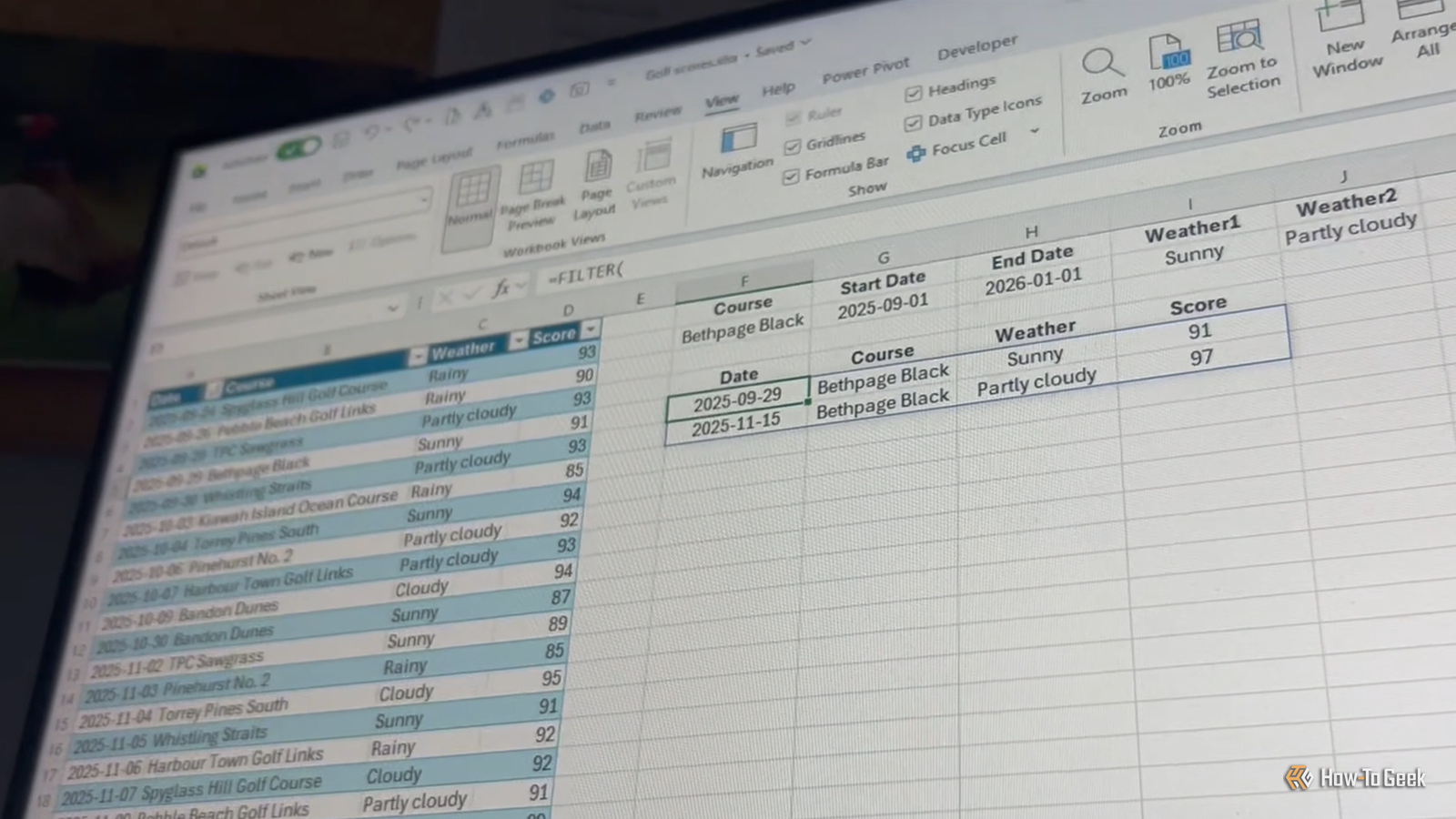
Published Sep 22, 2026, 7:00 AM EDT Tony Phillips is an experienced Microsoft Office user with a dual-honors degree in Linguistics and Hispanic Studies. Prior to starting with How-to Geek in January 2024, he worked as a document producer, data manager, and content creator for over ten years, and loves making spreadsheets and documents in his spare time. Tony is also an academic proofreader, experienced in reading, editing, and formatting over 3 million words of personal statements, resumes, reference letters, research proposals, and dissertations. Before joining How-To Geek, Tony formatted and wrote documents for legal firms, including contracts, Wills, and Powers of Attorney. Tony is obsessed with Microsoft Office! He will find any reason to create a spreadsheet, exploring ways to add complex formulas and discover new ways to make data tick. He also takes pride in producing Word documents that look the part. He has worked as a data manager in a secondary school in the UK and has years of experience in the classroom with Microsoft PowerPoint. He loves to encounter problems in Microsoft Office and use his expertise and legal-level training to find solutions. Outside of the Microsoft world, Tony is a keen dog owner and lover, football fan, astrophotographer, gardener, and golfer. If you've spent any time working with data in Excel, you've probably come across filtering. It's a quick way to focus on the records you need, analyze a subset of your data, and hide everything else from view. But Excel's regular filter buttons come with a few annoyances: they hide entire worksheet rows, can make the original dataset harder to see, and leave you with filters to clear when you've finished. That's where the FILTER function comes in. It creates a separate, live list of matching records, so your original data stays visible and untouched. And with a couple of nifty little tricks, FILTER is more flexible than you might first imagine. FILTER creates a separate, live list from your data Leave your source intact Credit: Lucas Gouveia/How-To Geek FILTER uses three arguments: =FILTER(array,include,[if_empty]) The first argument, array, is the data you want FILTER to return, whether that's a whole table, a single column, or several adjacent columns. The second, include, tells Excel which rows to include in the results. The optional third argument, if_empty, lets you specify what should appear if there are no matching records. FILTER works particularly well when your source data is an Excel table. Instead of pointing to a fixed range such as A2:D101, you can use the table's name and structured references, so the formula automatically picks up new rows added to the source data. There's one important catch: the FILTER formula itself needs to sit outside the Excel table. Its results spill into the cells below and beside the formula, and dynamic arrays can't spill inside a table. For this reason, make sure there's enough room for the results to spill, or Excel will return a #SPILL! error. Once that's set up, you can begin building your formula. Start with a single condition Let one cell control the results I use an Excel table named GolfData to keep track of my golf scores. Next to the table, I have a small criteria area with a data validation drop-down menu in cell F2 containing the course names. When I select a course, the FILTER function returns every round I've played there. I could hard-code the course name into the formula, but using a cell reference means I can change the criteria without editing the formula. In this case, F2 contains whatever course I've selected from the drop-down menu. Here's the formula: =FILTER(GolfData,GolfData[Course]=F2,"No rounds found") If you're building a formula with several criteria, press Alt+Enter as you type to insert a line break. The first argument tells FILTER to return the entire GolfData table, the second checks each row in the Course column against whatever I've selected in F2, and the third specifies the text I want to return if there are no matches. The result spills into the worksheet as a separate, live list, containing only the rows that match my selected course. Change the drop-down selection, and the list changes with it. Because FILTER creates a spilled range, I can also refer to the entire result from another formula using the spill range operator (#). For example, if my FILTER formula starts in F5, =ROWS(F5#) counts the number of records currently returned by the formula. Change the course in F2, and the count updates automatically. Add more conditions as your needs change FILTER can check several criteria A single condition is useful, but I can make the same formula more selective without starting over. This time, I've added start and end dates in G2 and H2. Now, I can filter the results to see rounds for my selected course that fall between those two dates. The good thing is that all I need to do is add those conditions to the existing formula: =FILTER(GolfData,(GolfData[Course]=F2) *(GolfData[Date]>=G2) *(GolfData[Date]=G2) *(GolfData[Date]=G2) *(GolfData[Date]<=H2) *((GolfData[Weather]=I2) + (GolfData[Weather]=J2)),"No rounds found") The + represents OR logic here, allowing either weather condition to return a match. So, for a row to be returned, it has to: Match the selected course, and Be on or after the start date, and Be on or before the end date, and Match either the weather selected in I2 or the weather selected in J2. This is why I like building FILTER formulas gradually. Once you understand what * and + are doing, you can create some quite specific result lists without manually filtering the source data over and over, hiding entire rows in your worksheet, or making your original data harder to see. Take FILTER to the next level I still use Excel's regular filter buttons when I want to hide rows temporarily. But when I want a separate, live list of the records that meet particular conditions, FILTER gives me a more flexible way to work. I can also combine it with other dynamic array functions like UNIQUE and SORTBY to create even more useful dynamic lists, taking the same live-list approach much further.