I replaced hundreds of Excel lookup formulas with this single tool

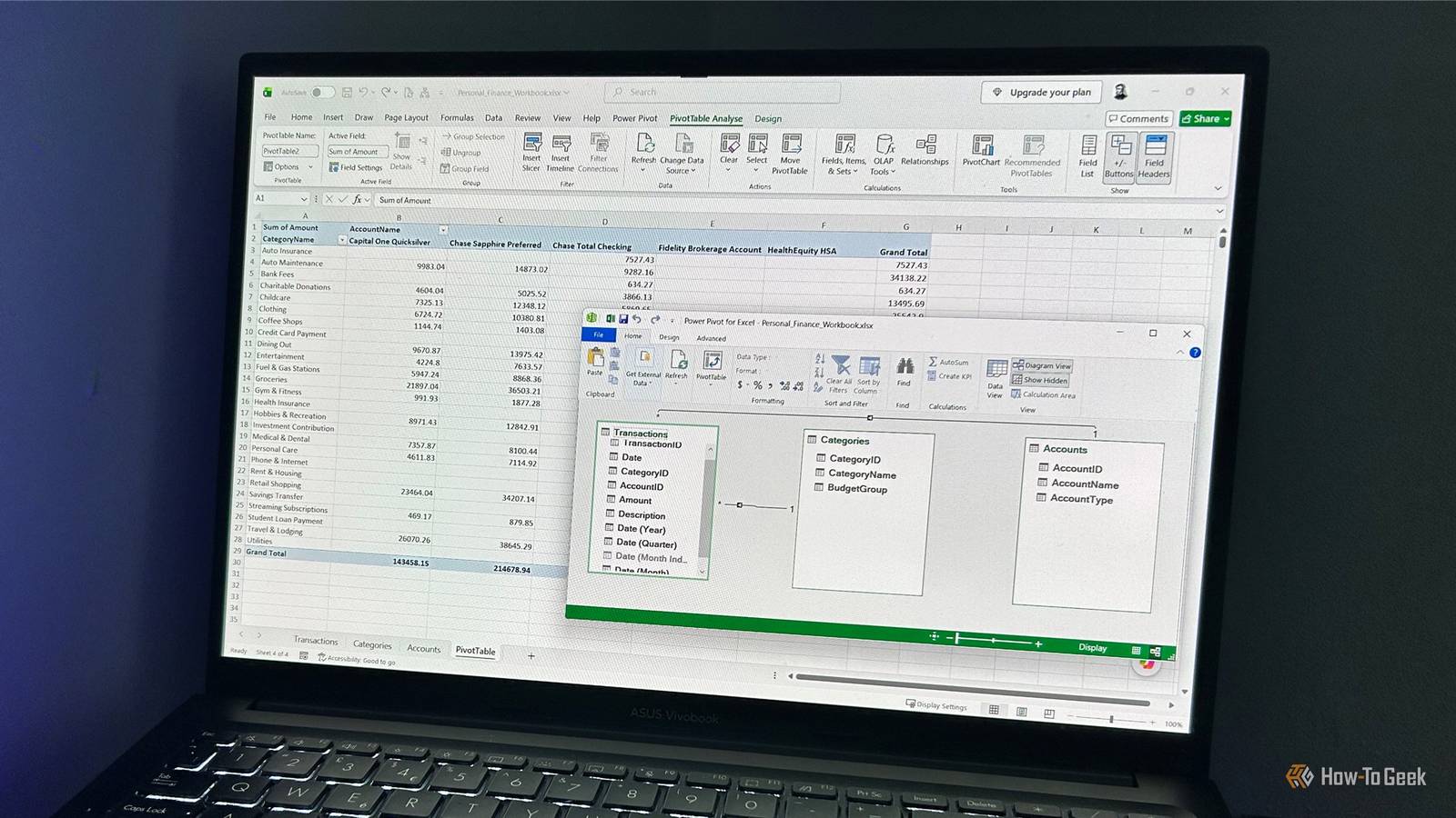
Published Aug 13, 2026, 6:30 AM EDT Tony Phillips is an experienced Microsoft Office user with a dual-honors degree in Linguistics and Hispanic Studies. Prior to starting with How-to Geek in January 2024, he worked as a document producer, data manager, and content creator for over ten years, and loves making spreadsheets and documents in his spare time. Tony is also an academic proofreader, experienced in reading, editing, and formatting over 3 million words of personal statements, resumes, reference letters, research proposals, and dissertations. Before joining How-To Geek, Tony formatted and wrote documents for legal firms, including contracts, Wills, and Powers of Attorney. Tony is obsessed with Microsoft Office! He will find any reason to create a spreadsheet, exploring ways to add complex formulas and discover new ways to make data tick. He also takes pride in producing Word documents that look the part. He has worked as a data manager in a secondary school in the UK and has years of experience in the classroom with Microsoft PowerPoint. He loves to encounter problems in Microsoft Office and use his expertise and legal-level training to find solutions. Outside of the Microsoft world, Tony is a keen dog owner and lover, football fan, astrophotographer, gardener, and golfer. I probably couldn't use Excel today without XLOOKUP. For quickly pulling information from one table into another, it's one of my most-used Excel functions. But as my workbooks grew, I found myself adding countless lookup columns and formulas just to make reports work. Power Pivot gave me a better way to connect my data. Power Pivot is available in Excel for Microsoft 365 and Excel 2016 or later on Windows desktop versions. It isn't available in Excel for the web. If you're using a supported desktop version but don't see the Power Pivot tab, enable it from File > Options > Add-ins, select COM Add-ins from the Manage dropdown, click Go, then tick Microsoft Power Pivot for Excel. My personal finance workbook started with three separate tables Excel workflows often start with one main table and a few smaller tables that link to it. In my case, I was working with a personal finance file containing thousands of transactions. The workbook had three tables, each on its own worksheet: The main Transactions table stored each purchase, including the date, amount, CategoryID, and AccountID. The Categories table contained labels for different spending categories, such as groceries, transport, and entertainment. The CategoryID column linked each category back to the Transactions table. The Accounts table stored details about financial accounts, such as Checking, Savings, and Credit Card accounts. The AccountID column linked those accounts back to individual transactions. The structure made sense. A category name only needed to exist once rather than being repeated across thousands of transaction rows, and each transaction only needed an AccountID. Credit: Tony Phillips/How-To Geek The challenge came when I wanted to build reports. Excel needed a way to connect each transaction with the information stored in the other tables. The traditional Excel approach creates a larger workbook XLOOKUP solves the problem by adding more columns My first solution was the one many Excel users would likely choose: add lookup columns to bring the missing information into the Transactions table. I copied the Transactions table into a fourth worksheet and added columns for CategoryName, BudgetGroup, AccountName, and AccountType. Then, I used XLOOKUP to pull in the data. For the CategoryName column, I entered: =XLOOKUP([@CategoryID],Categories[CategoryID],Categories[CategoryName]) In BudgetGroup, I used: =XLOOKUP([@CategoryID],Categories[CategoryID],Categories[BudgetGroup]) For AccountName, I typed: =XLOOKUP([@AccountID],Accounts[AccountID],Accounts[AccountName]) And in the AccountType column, I entered: =XLOOKUP([@AccountID],Accounts[AccountID],Accounts[AccountType]) This worked exactly as expected, and I could now create a PivotTable in a fifth worksheet. For example, I could add CategoryName to the Rows area, AccountName to the Columns area, and Amount to the Values area to see how much I spent in each category across my different accounts. But the problem wasn't functionality. It was the workbook structure. I'd gone from three clean tables to a workbook containing the original Transactions table, the Categories and Accounts tables, a second Transactions table with repeated information, and a PivotTable worksheet for reporting. In essence, I had created extra data and worksheets just so Excel could understand how the tables were connected. Power Pivot connects Excel tables without adding lookup columns The Data Model lets Excel understand relationships Instead of combining the tables first, Power Pivot lets me keep them separate and tell Excel how they are related. I loaded my three tables into the Data Model by selecting each table, opening the Power Pivot tab, and choosing Add to Data Model. Then, I opened the Power Pivot window, switched to Diagram View, and connected the matching ID fields to create relationships: Transactions[CategoryID] → Categories[CategoryID]Transactions[AccountID] → Accounts[AccountID] Once I'd set those up, Excel understood how the tables were related. I could then create the same PivotTable report directly from the Data Model, with CategoryName as rows, AccountName as columns, and Amount as the value to see how spending was split across categories and accounts. The result was the same spending report I created using XLOOKUP, but the difference was how I got there. With XLOOKUP, I had to add category and account information to thousands of transaction rows before creating the report. With Power Pivot, the original tables stayed separate, and Excel used the relationships between them when building the PivotTable. The information stayed where it was, and I avoided creating another copy of my transactions data. Pro tip: Power Pivot adds PivotTable features you don't get elsewhere Keeping my workbook tidy is the main reason I started using Power Pivot, but the Data Model also unlocks features that aren't available in PivotTables built directly from worksheet ranges or tables. One example is Distinct Count, which appears as a built-in summary option in the Value Field Settings dialog. If your aim is to cut down on helper formulas and summary tables, that's another good reason to try Power Pivot. XLOOKUP works—until your workbook needs a different structure XLOOKUP is still one of my favorite ways to bring information together in Excel, especially in smaller workbooks. But when my data is split across multiple related tables, Power Pivot gives me a cleaner way to build reports without first combining everything into one larger table. If your version of Excel doesn't support Power Pivot, however, Power Query can help you create a similar reporting workflow by merging related tables, appending data from multiple sources, and automating the creation of a clean reporting table.