I ditched multiple Excel worksheets for one dynamic report and saved myself a ton of work

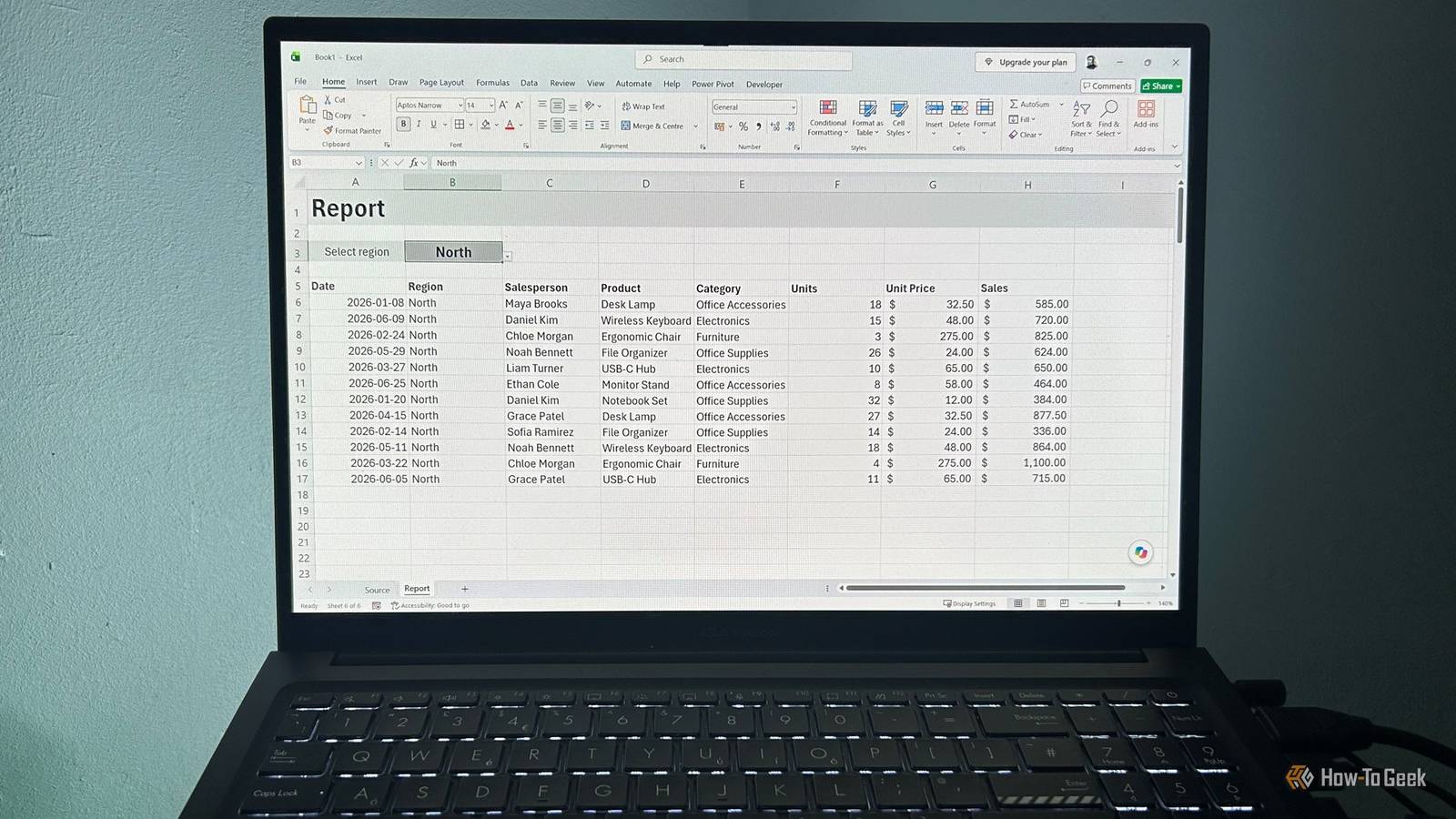
Published Oct 6, 2026, 10:30 AM EDT Tony Phillips is an experienced Microsoft Office user with a dual-honors degree in Linguistics and Hispanic Studies. Prior to starting with How-to Geek in January 2024, he worked as a document producer, data manager, and content creator for over ten years, and loves making spreadsheets and documents in his spare time. Tony is also an academic proofreader, experienced in reading, editing, and formatting over 3 million words of personal statements, resumes, reference letters, research proposals, and dissertations. Before joining How-To Geek, Tony formatted and wrote documents for legal firms, including contracts, Wills, and Powers of Attorney. Tony is obsessed with Microsoft Office! He will find any reason to create a spreadsheet, exploring ways to add complex formulas and discover new ways to make data tick. He also takes pride in producing Word documents that look the part. He has worked as a data manager in a secondary school in the UK and has years of experience in the classroom with Microsoft PowerPoint. He loves to encounter problems in Microsoft Office and use his expertise and legal-level training to find solutions. Outside of the Microsoft world, Tony is a keen dog owner and lover, football fan, astrophotographer, gardener, and golfer. It's easy to end up with multiple versions of the same Excel report. You might need one for each region, department, or product, so you copy the report and change the data it shows. I've done this plenty of times, and for a while, I didn't see much of a problem. Then I realized I was maintaining several reports that were basically doing the same job. I came up with a way to keep those different reports while maintaining just one, and it has saved me a ridiculous amount of repetitive work. Multiple Excel reports work fine—until you have to change one Four reports walk into a maintenance problem In theory, there's nothing "wrong" with having multiple versions of the same report scattered across worksheets in an Excel workbook. You might have North on sheet 1, East on sheet 2, South on sheet 3, and West on sheet 4, all dynamically linked to a source worksheet with formulas that update when the underlying data changes. And that all works fine. The problem is that you now have four copies of the report to maintain. If you change the formatting, add or move a column heading, or add a total row, you have to make the same change four times. Add a new column to the source data, and you'll then need to apply the right number format to that column on all four reports. One Excel report can replace the whole collection Give the report a little decision-making power The trick is to have one FILTER formula use a cell value to control what it displays. Instead of creating separate worksheets for North, East, South, and West, I can put those choices into a drop-down list and let Excel decide which records to display. I'll use a sales table called tblSales, which contains a Region column. Make sure your source data is formatted as an Excel table. This lets the formulas use structured references like tblSales[Region] and automatically include new records as they're added. If your data is currently a normal range, select it and press Ctrl+T. My report has the same layout I want to use for every region, but instead of building four versions, I'll create just one additional Report worksheet and add a data validation drop-down list to cell B3. If the table and the drop-down are on the same sheet, a direct reference to the column's cells expands automatically as the table grows. Because mine are on separate worksheets, I created a named range for the column instead (Formulas > Name Manager > New). Excel for Microsoft 365 automatically removes duplicate values from this type of data validation list. If your version doesn't, use UNIQUE to create a separate list of unique regions, and use its spilled results as the data validation source. For example, if UNIQUE is in H2, use =$H$2# as the source. I can now select cell B3 in my Report worksheet, go to Data > Data Validation, choose List, and use that name as the source in the dialog. Now I have my selector. The next job is to make the report respond to it. That's where the FILTER function comes in. In the first cell where I want the results to appear, I enter: =FILTER(tblSales,tblSales[Region]=B3) Make sure there are no existing values in the cells where the results need to spill, or Excel will return a #SPILL! error. The first argument tells Excel what data I want returned, while the second tells it to return only the rows where the Region column matches the selection in B3. Compare that to the formula I used to create one-off, separate reports for each region. The hard-coded criterion means each formula can only show data for its designated region: =FILTER(tblSales,tblSales[Region]="North") Now, if I change the drop-down selection to East, the results update straight away. I haven't created another report or changed the formula—the selection is doing the work. And crucially, if I need to change the report's layout, formatting, or totals, I only have to make the change once instead of four times. If you need totals or counts rather than the actual records, a PivotTable with a slicer is the better tool, but for listing the matching rows in a layout you control, a drop-down list and the FILTER function win. Make one report handle multiple conditions Go beyond a single drop-down list Once I had one cell selection controlling my report, I realized how much more useful this approach became when I added another criterion. With the old setup, reports that varied by both region and product could quickly turn into a worksheet for every combination: North/Desk Lamp, North/Standing Desk, East/Desk Lamp, East/Standing Desk, and so on. Add more regions or products, and the number of possible reports multiplies rapidly. With the dynamic version, all those combinations can live on the same Report worksheet. I can add a second drop-down and let FILTER handle both selections, rather than creating another worksheet for every possible combination. Let's say B3 contains my selected region and D3 contains my selected product. I can use both selections in the FILTER formula: =FILTER(tblSales,(tblSales[Region]=B3)*(tblSales[Product]=D3),"No matches") The asterisk (*) between the two conditions means AND, so Excel returns only the records where both conditions are true. This is where the "No matches" argument becomes useful. My drop-downs might contain valid regions and products individually, but there might not be any records for that particular combination. For example, I could select North and Standing desk, even though tblSales contains no North sales for that product. Instead of returning an error, the report displays "No matches." I can also use a plus sign (+) when I want OR logic. For example, if B3 and D3 contain two regions and F3 contains a product, this formula returns records for either region, but only for the specified product: =FILTER(tblSales,((tblSales[Region]=B3)+(tblSales[Region]=D3))*(tblSales[Product]=F3),"No matches") And I can keep adding criteria and selectors as the report requires, without multiplying worksheets. That's the real benefit of this approach. Let Excel do the spilling Excel's spill behavior is what makes this approach work. Instead of creating a separate formula and report for every variation, one formula can return an entire set of matching records and automatically resize the results as my selection changes. FILTER is only one of Excel's dynamic array functions that can work this way. Other dynamic array functions can use the same spill behavior, so once you combine them with cell-driven selections, you can start replacing other collections of repetitive reports with a single dynamic version.