How to Optimize Vector Search When RAM Gets Too Expensive: On-Disk vs. In-Memory ANN Indexes

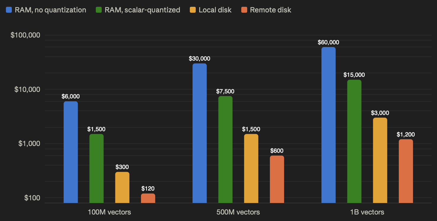
, vector search has become a critical piece of AI infrastructure, powering use cases from RAG and semantic search to agentic memory and context layers. With the rise of agentic systems, companies are trying to provide as much context to the agents as possible, which requires vector db indexes to grow from an initial million or dozens of millions scale to the hundreds of millions or even billions. At this scale, storing indexes and associated data in RAM will cost thousands of dollars per month, and HNSW can become a scalability bottleneck. In this article I would like to dive into the details of what actually makes semantic search fast and efficient: approximate nearest neighbor (ANN) algorithms, what different options exist, and their trade-offs. Deep dive into vector DB Vector databases consist of three main components: embeddings – the numeric representation of the corpus search algorithm and index structure – the algorithm defines the search quality and speed storage – how the data is stored (in memory, on disk, payload together with embeddings, etc.). Whether in RAM or on disk, it determines the costs and latency at scale Embeddings are already well defined and discussed in many articles, and this one will focus on search algorithms, and specifically ANN ones. There are generally two approaches for the search execution: Exact search – which demonstrates the best retrieval metrics although it does not scale well in terms of latency Approximate nearest neighbor (ANN) – which trades off the retrieval quality for the latency and scalability. The exact search is a simple approach which loops through all of the entries in the index and calculates the distance between your search query and existing data. There are no losses related to any approximation or generalization with the trade-off of the latency and scalability. It’s a great approach for either very small indexes or experimentation, but generally not very suitable for the production scale. Interesting fact: many modern vector databases allow you to bypass index building for small collections, falling back to kNN search because the overhead of building an index is not worth it for a few thousand vectors. The second option is approximate nearest neighbor algorithms, which is a group of algorithms with the main purpose of improving scalability by avoiding visiting all the entries in the index. The idea here is to provide some shortcuts to speed up the search and ingestion. The implementations vary, although many modern ANN algorithms (for example, HNSW and DiskANN) rely on a graph structure to provide low query latency. Approximate nearest neighbor algorithms It’s important to discuss that even though ANN algorithms are all following a similar concept to achieve the goal of providing a short path to the end result, there are different implementations with different algorithms having unique sets of trade-offs, which makes it crucial to select the one that fits your exact use case. In this article I would like to focus on two different groups of the ANN algorithms: RAM-based – such algorithms are optimized for storing all or a big chunk of data in memory, which provides extremely low latency with the costs as a trade-off. The standard example here is HNSW (Hierarchical Navigable Small World) On-disk – these algorithms are minimizing RAM usage and relying heavily on disk to load the required data. An example here is DiskANN or SPANN It’s required to mention that it’s possible to store underlying data structures of both of these algorithm groups either on disk or in memory (at least partially), but they are optimized for the specific storage type and therefore will provide the best results utilizing what they were designed for. In-memory ANN HNSW (Hierarchical Navigable Small World) HNSW’s layered graph: a query enters at the sparse top layer, greedily walks to the nearest node, then drops down and repeats until the dense bottom layer. Image by author. The most popular ANN algorithm used by almost any modern vector database. The idea is to utilize a layered graph-based data structure to connect vectors with near neighbors, which provides extremely fast retrieval when storing the whole index in memory. It’s a great fit for small-medium use cases and will provide the best retrieval speed. However, once the index is big enough that it no longer fits in RAM or storing it in RAM becomes very expensive, the option is to either move data to disk, which may cause a drastic performance hit, or highly quantize it, which can cause a significant drop in retrieval quality. The main reason for such a performance hit is that the HNSW structure is not optimized for the clustered disk access, and as a result, the search would produce a lot of non-sequential I/O operations. Considering multiple hops per search and relatively high read traffic, the disk I/O will become a bottleneck, which can significantly increase latency, from milliseconds to hundreds of milliseconds or worse under heavy I/O pressure. The in-memory algorithms are highly optimized to store all vectors and connections in RAM, which makes them extremely fast, but with a trade-off of being memory hungry. Moreover, with on-disk options such algorithms rely on random disk access, which can become a potential bottleneck for large-scale indexes (100 million+). Example vector databases: Qdrant, Milvus, pgvector, OpenSearch, Weaviate, Redis On-Disk ANN This group of algorithms is designed specifically to break the RAM consumption limitation of the in-memory ANN algorithms and reduce the storage costs while providing acceptable latency. It’s a great choice if search latency is not critical and the index size is expected to be large. We can consider two main algorithms in this group: SPANN SPANN’s routing layer: centroids stay in RAM, the vectors they represent are stored on disk. Image by author. It’s a disk-based ANN algorithm that follows the inverted-index (IVF) methodology: vectors are grouped into clusters, each represented by a centroid. It was specifically designed to handle extremely large billion-vector+ indexes that won’t fit in RAM or will be too expensive to be stored in memory. The idea is to organize points in clusters, which is a natural property of the embedding space, select a centroid representation of the cluster, and utilize it for the routing layer. Centroids and basically the whole routing layer can be stored in RAM while the vectors represented by the centroids are stored on disk. The important detail is that vectors represented by the same centroid are stored on disk sequentially and therefore can be loaded from it fast and efficiently. During search, centroids are used to find the closest groups of vectors, and then the vectors associated with those centroids are loaded from disk to perform a full scan. Note: Compared to HNSW with the on-disk storage option, SPANN ensures that instead of random disk access, the vectors represented by the single centroid are grouped on disk and therefore loaded as blocks, which dramatically reduces the number of required disk I/O operations while providing acceptable latency. Example vector databases: Turbopuffer (built on SPFresh, a SPANN successor), Chroma DB (cloud) DiskANN DiskANN’s layout: quantized vectors and the graph are kept in RAM, the full-precision vector is read from disk for each visited point. Image by author. Instead of a centroid-based approach, DiskANN maintains a single-layer graph called Vamana. The main idea behind it is to minimize the number of hops required to find the top k points and therefore the number of random disk access operations. It’s achieved by keeping some longer-range connections instead of only the nearest ones, so fewer hops are needed to reach the target. The original vectors are stored on disk while the highly quantized version of the vectors is stored in RAM, which also contributes to reducing the required number of disk access operations. Compared to SPANN, DiskANN’s Vamana graph is built over every point, so the graph itself scales with the dataset, which is a real memory consideration at billion scale, where SPANN only needs its centroids resident. The data on disk is not clustered, and the disk I/O is minimized by the routing layer doing a minimal number of hops to get to similar vectors, leading to highly efficient search in practice. There are a lot of internal details on how exactly it’s implemented, and I highly recommend exploring the origin paper, which is linked in the references for this article. Example vector databases: Milvus, PostgreSQL (via pg_diskann) Economics Note: the prices below are approximate and current as of writing. Cloud pricing shifts over time and varies by provider, region, and commitment, so treat these figures as illustrative of the RAM-vs-disk ratio rather than exact quotes With RAM costing about 5$ per GB through cloud providers, EBS is about 50 times cheaper, around 0.08-0.10$ per GB, and local NVMe SSD around 0.20-0.25$ per GB. Therefore, for the 100,000,000 index in 1024 dimensions with float32 precision, it will be 1024 * 4 bytes = 4 KB per vector, and with production-grade replication of 3 it will require 12 KB of storage per vector. Therefore, for 100,000,000 vectors, the total required amount of storage is 1.2 TB. Of course, there is a quantization option, which will reduce this number, and the most popular and least invasive scalar quantization will require 25% of the storage, which is 300 GB. Therefore, the approximate monthly storage associated costs: Non-quantized in RAM ~6000 USD Scalar-quantized in RAM ~ 1500 USD Remote Disk ~120 USD Local Disk ~ 300 USD And because this is a linear relationship, the gap only widens as the index grows toward the scale agentic systems are pushing toward: VectorsStorage (non-quantized)RAM cost/monthScalar-quantized RAM cost/monthRemote Disk cost/monthLocal Diskcost/month100M1.2 TB~6,000~1,500~120~300500M6 TB~30,000~7,500~600~15001B12 TB~60,000~15,000~1,200~3000Table 1: Approximate monthly storage costs, excluding compute, across index sizes and storage tiers. Image by author As a result, even though scalar quantization reduces the bill significantly, it’s still a high cost compared to the on-disk option. The trade-off As with everything in engineering, the cost reduction provided by on-disk ANN algorithms is not free. While the routing layer does ensure efficient data retrieval and narrows down the exploration to the smaller subset, the data still needs to be loaded from the disk, which is significantly slower than loading it from RAM. It’s worth mentioning that for a lot of use cases it may not be a deal breaker. Considering cases such as RAG, where results from the vector db are then passed to the reranker and LLM, the 100ms delay on the retrieval is not going to be the main bottleneck, but for cases such as agentic memory, context, etc., it actually may be preferred to be able to execute search as fast as possible, specifically if there are multiple calls during a single agent request processing. It’s genuinely hard to give a clear number for on-disk latency, and that’s sort of the point, it highly depends on the exact setup. For example, the SPANN paper reports reaching 90% recall in around 1ms at billion scale, but that’s a mean latency on a single machine with the index stored on local SSD. Once you move to a real deployment, the picture changes. Turbopuffer’s benchmark on a 10M-vector index shows around 14ms at p50 when the index is warm on fast storage, but close to 874ms when it’s cold and has to be fetched from object storage, which is around a 60x difference on the same data just from the cache state. Factors like hardware and whether the data is warm (already in cache) can each move the number by 10x or more. General guidance is that disk-based ANN algorithms provide slower latency than HNSW (in RAM) just because RAM access is much faster. Choose wisely With both on-disk and in-memory algorithms, it’s important to make the right choice about which one will be a better fit for your use case. While HNSW provides an easy, well-rounded solution for small and medium size indexes, it may be worth exploring the on-disk options once your index grows bigger and the associated costs of storing vectors in RAM become a burden. Moreover, there are always edge cases like relatively high-dimensional vectors for which RAM will be a bottleneck relatively early or huge low-dimensionality indexes which can utilize RAM for much longer. For engineers, it’s important to be aware of such use cases and make a comprehensive decision on the trade-offs appropriate for their use cases. AlgorithmWhat stays in RAMLatencyScales to Reach for it when Exact searchFull vectors (or streamed from disk) grows with N< ~10ktiny collections, ground-truth evalHNSWwhole index (disk possible, big latency penalty)often in sub 10ms~1M–100M in RAMlatency-critical, index fits RAM budgetDiskANNPQ vectors + graph; graph grows with Nlow ms warm, slow when cold100M–1B+large & cost-sensitiveSPANNcentroids only low ms warm, slow when cold100M–multi billionseven PQ-in-RAM is too expensiveTable 2: Summary of ANN algorithms by RAM footprint, latency, and practical scale. Image by author. References HNSW paper https://arxiv.org/abs/1603.09320 SPANN paper https://arxiv.org/abs/2111.08566 DiskANN paper https://papers.nips.cc/paper_files/paper/2019/hash/09853c7fb1d3f8ee67a61b6bf4a7f8e6-Abstract.html TurboPuffer performance: turbopuffer.com/tldr