Dynamical System Transfer Learning with Reduced Order Models

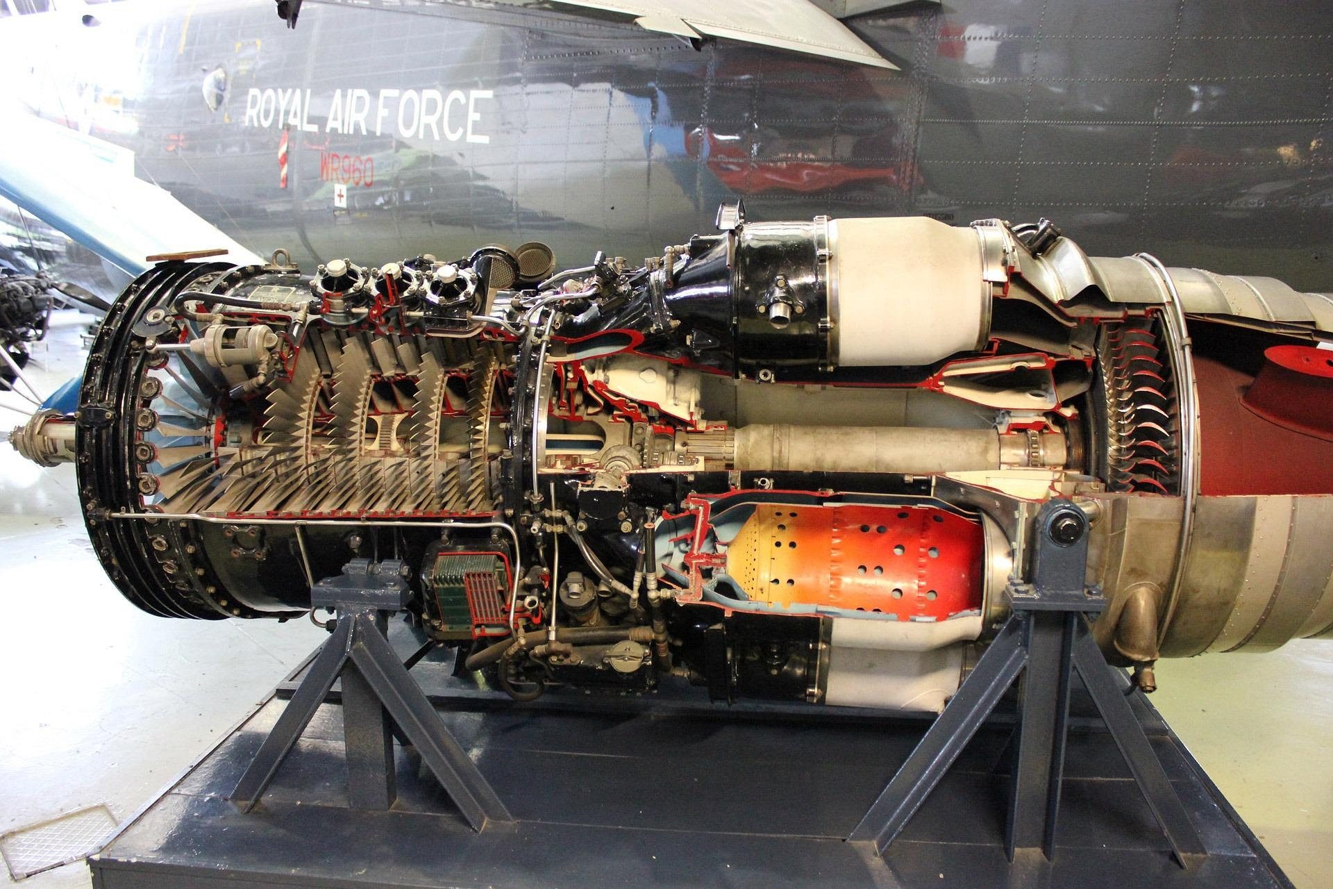
I have discussed previously the potential utility of applying Reinforcement Learning (RL) to analysis and control of complex physical systems. Developing RL algorithms to analyze or control complex dynamical systems faces one of the main challenges of many other RL problems — lengthy training times. This problem is complicated by the high computational cost of simulating complex physical dynamics. Compounding the thousands (perhaps millions) of RL training iterations needed for large state spaces and nonlinear systems with simulation times that may run into the hours (or even just minutes) per iteration can make problems intractable. Transfer learning has been used to reduce training times for RL problems and here we will explore application of transfer learning to RL for dynamical systems.Transfer learning relies on using models trained on similar problems to reduce training time with the assumption that the problem is similar enough that the model will have to make only small changes. For example, using an RL algorithm trained to drive a small RC car will probably more quickly learn how to drive a tractor trailer than one starting from scratch despite the considerable difference between the two. Reduced Order ModelsFor physics simulations we need a problem environment to train the RL algorithm on that will be similar enough but substantially faster to simulate than the original. Reduced Order Models (ROMs) provide a way to generate such environments. A ROM, at its simplest, is a simplified model that seeks to reduce complexity while retaining as much accuracy as possible. There are many ways to generate ROMs. Any AI can be considered a ROM, from supervised learning to even large language models as ROMs of human language. Here we will apply unsupervised learning based on an approach outlined in Brunton and Kutz’s book Data Driven Science and Engineering to develop a data-driven ROM of a physical dynamical system based only on a data set of system measurements with little knowledge of the underlying system.As a brief introduction, dynamical systems are those that can be described as evolving through time. They are often summarized asdx/dt=F(x)d\mathbf{x}/dt = F(\mathbf{x})where x is the state vector (set of variables that describe the system), dx/dt is the change in state with the change in time, and F(x) is some function of the state variables (sometimes including their history). The state vector x can be one variable or thousands, especially when state history is needed. F(x) may be a linear or nonlinear system. Linear systems have predictable response to input—double the input, double the response. Nonlinear systems, far more common and representative of the real world, do not exhibit that behavior throughout all possible states. Doubling input may double output, multiply output by 100, or drive output to 0, and this behavior can change depending on where you are in the state space (region of all possible values the variables can take). Real-world physical systems exhibit nonlinearity making them difficult to characterize. On top of that, realistic physical and engineering systems often lack solvable, direct, comprehensive governing equations that would support analysis of their behavior. The equations we can obtain, much less solve, often require simplification that constrict their utility to a subregion of the state space or lose track of higher order dynamics. Consider turbojet engine dynamics (which will be our example problem): the simulation we will use is based on a series of coupled equations that must be solved iteratively rather than directly solving a dynamic system of equations. Even then, it contains many simplifications of the coupled fluid, structural, thermodynamic, and chemical processes at work. Typical approaches, such as linearization around known solutions and creative use of coordinate systems, have become less helpful as complexity and scope of systems under analysis increase. However, as system complexity has exceeded traditional analytical approaches, our ability to gather, store, aggregate, and analyze measurement data at GB, TB, and even PB level has improved.Brunton and Kutz’s text discusses new techniques to approach dynamical systems exploiting increased measurement, storage, and analysis capabilities. Their approaches are based on unsupervised learning—that is looking for underlying patterns without a priori knowledge of what those patterns should be. These techniques use measurements of system state over time to derive dynamic models that can be used to describe, analyze, and predict behavior. The particular method we will use here is SINDy (Sparse Identification of Nonlinear Dynamics).Sparse Identification of Nonlinear Dynamics (SINDy) The goal of the SINDy algorithm is to discover system models in the form of mathematical equations using system measurement data, specifically a time series of state data that can be used to calculate an array of time derivatives of state variables over time. Essentially, it takes a candidate library of possible equation terms (such as products, quotients, and derivatives of states) and determines a parsimonious equation (that is, one that uses the fewest number of terms) that best describes the state changes over time. The basic equation describing SINDy is:dx/dt=θ(x)Ξd\mathbf{x}/dt = \theta(\mathbf{x})\Xiwhere Θ(x) is the array of possible equation terms and Ξ is a matrix of coefficients for those terms. For example, if the equation exhibits strong quadratic behavior but no sinusoidal, then the value in Ξ corresponding to the quadratic vector of Θ(x) will have a large absolute value and the value corresponding to the sinusoid will be near 0. For more details, see the original SINDy paper: https://arxiv.org/abs/1509.03580 or a tutorial video: https://www.youtube.com/watch?v=gSCa78TIldg. The SINDy algorithm has been able to identify complex fluid flow models just from time series data. Here we will see how well it can discover dynamic equations describing a turbojet engine (or at least describe the simulation we are using). Turbojet Modelling The specific problem here is creating an autothrottle for a turbojet engine. We want our RL algorithm to adjust the throttle on a turbojet engine to achieve a 10% change in speed at a given altitude, balancing time to new speed against fuel use. This is not a problem that would typically require reinforcement learning; autothrottle systems based on classical control, gain scheduling, or other techniques have been around for decades. Further, these other approaches have the advantage of being deterministic and so easier to certify for flight operations. Hence, I am not proposing this as a practical application of RL but chose it for convenience to illustrate the principles of (1) using RL on complex physical systems and (2) generating ROMs of complex physics as a source for transfer learning.Engines are the most complicated parts of an aircraft; generally speaking, the engine is about as hard to design as the rest of the aircraft. Solving for engine performance involves both aerodynamic and thermodynamic equations, both with rich and complex nonlinear behavior. I chose the turbojet problem specifically because of the complex physics and the availability of a reasonably high-fidelity model in Python. Turbojet engine operation is characterized by a balance of air and fuel mass flow, energy conservation, pressure ratios, non-constant gas dynamics, and other factors. Determining jet engine performance requires iteration—assume a set of gas properties such as density, pressure, temperature, velocity — at each of 6 or more stages through the engine, determine resulting mass flow and thermodynamics at each stage, and then iterate by adjusting assumptions for inlet mass flow, fuel flow, etc. until solution converges for particular operating parameters (speed in Mach number, altitude, and throttle setting). The Flight Test Engineering Github provides a jet engine simulator (along with an accompanying YouTube tutorial series) that allows definition of a jet engine and then simulation of its performance across a range of operating parameters. To account for variations in altitude and air compressibility, this simulation uses the ISA tools Python library which contains functions that translate altitude, temperature, density, speed, and Mach number based on the standard atmosphere. We will use this simulation as the foundation of a training environment for the baseline (non-transfer) RL algorithm and to provide the basis for a ROM. Even the “full” simulation used here is drastically simplified. Doing a full computational fluid dynamics model of even a small section of a jet engine takes tens of thousands of computational hours (and even that will contain substantial simplifications and assumptions about small-scale fluid dynamics and turbulence). Aircraft dynamicsTo match throttle setting to velocity change, we need to develop a basic aircraft model. We will use basic aerodynamics for a hypothetical aircraft that our engine will power. The RL algorithm will have to “learn” the drag behavior of this aircraft to properly set the throttle, with the drag in turn defined by aircraft aerodynamics. The aerodynamic parameters defining the aircraft and engine will be selected to provide realistic results. First, we define the engine. The turbojet simulator can design engine parameters such as compressor, combustor, and turbine given basic geometric parameters and a design point. We will define our engine around the performance of the J-47 used to power the B-47 Stratojet bomber. The B-47 had six engines, so we choose aerodynamic parameters at a scale of 1/6 of the B-47 and adjust from there for realistic performance, providing the following parametersm (mass)10000 kgCd0 (parasitic drag coefficient)0.0148AR (aspect ratio)5.0S (wetted surface area)22.2 m^2e (Oswald efficiency)0.85Next we need to define the aircraft dynamics based on these parameters. We will discretize the system and evaluate at each 0.1 s the current acceleration based on engine thrust and drag. We start from Newton’s second law to relate force to change in velocity. Force is determined by thrust (provided by the engine simulation or ROM) and drag (calculated from basic aerodynamics). F=T−D=m∗dv/dtdv/dt=(T−D)/mdiscretizing yields(v1−v0)∗dt=(T0−D0)/mT (thrust) from python engine simulationD(drag)=1/2ρ v2 S Cd whereCd (drag coeficient)=Cdi+Cd0Cdi (induced drag)=Cl2/(πeAR)Cl (liftcoefficient)=m/(1/2∗ρ∗v2∗s)F=T-D=m*dv/dt \newline dv/dt = (T-D)/m \newline discretizing\: yields \newline (v1-v0)*dt = (T0-D0)/m\newline T\:(thrust)\: from\: python\: engine\: simulation \newline D (drag) = 1/2\rho\: v^2\: S\: Cd\:\: where \newline Cd\: (drag\: coeficient) = Cdi + Cd0 \newline Cdi\: (induced\: drag) = Cl^2/(\pi e AR)\newline Cl\: (lift coefficient) = m/(1/2 *\rho*v^2*s) Density, ρ, is determined from state altitude using ISA library. V (velocity) is determined from state Mach number using ISA library. At each time step dt = 0.1, we calculate current thrust and drag and add resulting acceleration to current velocity to determine new velocity to a first order approximation.Developing the RL algorithmsStable Baselines provides the RL algorithm; in this case we will use PPO as it is a popular, accurate, stable algorithm applicable to continuous action spaces. Information on PPO is available on Stable Baselines' documentation. Stable Baseline algorithms are designed to work with the gymnasium interface, so I have created a gymnasium based on the turbojet simulation. Most of the turbojet script was condensed into a local library called by the “TJ” custom gymnasium environment. A Jupyter Notebook walkthrough training each model and development of the SINDy ROM is available on Github.The RL algorithm takes as input the state (agent location) of altitude, Mach number, and target Mach number and returns action of throttle setting. In the step function, the gymnasium uses the throttle setting action to run the turbojet simulation and determine a new thrust and fuel flow. Commented step function for the gymnasium is is shown below; full code for the gymnasium is available on Github.It uses the new thrust and current state to calculate drag and new velocity over the 0.1 s time step. The ISA library converts velocity back to Mach number, the step function compares to target Mach, and gives a (negative) reward based on fuel flow. If achieved Mach is close to target Mach, then the run is done and the algorithm stops decreasing its reward with fuel flow. If velocity comes close to unphysical (negative) values the run truncates with large negative reward. We train the PPO algorithm using Stable Baselines interface for 5000 total timesteps and observe the reward obtained as total time elapses.SINDy-based ROMAs discussed above, the ROM is based on SINDy. The dynamical system is as described above—dv/dt = 1/m (T-D), where the nonlinear dynamics are contained within the Thrust function T. To provide the data array SINDy requires, we use the turbojet simulation code to generate an array of Mach-altitude-throttle setting-thrust data. We add to this data dv/dt corresponding to each state based on the aircraft dynamics above. This provides the data needed by the SINDy algorithm. We could just use the look up table to match throttle setting to thrust but take this approach to demonstrate use of SINDy-based ROMs for dynamical systems. To apply SINDy we use the python SINDy library (https://pysindy.readthedocs.io/en/latest/index.html) which includes candidate function term generators for polynomial, sinusoidal, and exponential terms. The library requires an input data table containing the state dynamics of the system and will generate a model based on the selected suite of candidate terms. Interestingly, the resulting equation:dv=−3.022+1.973∗Throttle−0.132∗Throttle3dv=-3.022+1.973*Throttle-0.132*Throttle^3does not include altitude or Mach number. Under the current simulation and aircraft model, SINDy considers them non-factors in the ROM. The absence of altitude isn’t a huge concern since altitude lowers thrust but also drag, and turbojet engines are more resilient to loss of density than turbofan or piston. The absence of Mach number is more concerning; turbojet engines typically produce thrust roughly constant with velocity but drag increases with velocity. The performance of the transfer learning algorithm on the full simulation will tell us if this is a reasonable assumption.Transfer Learning RL algorithmThe transfer learning approach requires first training an algorithm on the ROM, which requires the ROM to be embedded within a gymnasium: TJ_Rom. This gymnasium has the same state and action spaces as the gymnasium for the full turbojet simulation. However, instead of the turbojet simulation elements it has the SINDy-derived equation for dv based on throttle setting in the step function. Also, instead of building a model for fuel flow, scaled throttle setting is used as the (negative) reward under the assumption that fuel flow will closely scale with throttle setting. Commented step function code is given below; the full gymnasium is available on Github.Training on the ROM gymnasium is run on the same PPO algorithm as for the full simulation but for 10000 total timesteps. The resulting model is saved and then used for 5000 total timesteps on the full simulation. To evaluate the success (or failure) of transfer learning, we compare the reward at different total time elapsed. To calculate time elapsed for the non-transfer learning we take elapsed time straight from model output while for transfer learning we add ROM training time to elapsed time for the full simulation run. We don’t need to complete training to high accuracy to compare the performance of the baseline vs transfer learning. To save CPU time (and frustrating crashes from memory limits on my 5 year old mid-line laptop), I limit iterations to compare early stage reward progress between the two. The ROM training was much faster than full simulation: 13 seconds for 10000 time steps vs about 2500 seconds at 4000 timesteps for the full simulation. After 2596 seconds computing, the baseline ROM had achieved reward of -2080, while at 2232 seconds the transfer learning ROM achieved -1170. We see that the ROM is effective at reducing training time for the full problem.ConclusionReducing training time needed to apply RL to complex physical systems provides opportunity to apply RL to a wider range of problems. As we discussed, RL’s utility to this specific problem is limited; jet engine autothrottles can use existing control techniques to provide adequate performance. However, given how nonlinear systems can contain unknown or unexpected operating conditions, applying RL even to systems with existing control approaches may help us find new, more efficient operating modes or design points or may provide more robust and flexible control systems that could take over if the design conditions for traditional controllers are exceeded. For more complex systems where existing control approaches are overly constrictive or inadequate, RL may provide new advances.Further, the SINDy approach used for ROM generation here, and similar data-driven engineering approaches, can help provide insight and capture behavior of systems that were previously too large or complex to model effectively. The resulting ROMs can be used for classical analysis and control techniques, used to augment RL or other AI approaches as here, or used to aggregate models and simulations to get past scaling or stiffness problems that hinder analysis (such as material responses to and impact on aerodynamic and nuclear dynamics).Note: Throughout we used low order approximations in discretization and aerodynamic calculations. We even disregarded shock drag as the domain for the gymnasium includes compressible Mach numbers. The goal, as mentioned, was not to create a functional RL-based autothrottle but to demonstrate the principle and utility of (1) the SINDy method to create ROMs of physical dynamical systems and (2) reducing RL training time by using those ROMs for transfer learning, a goal we accomplished with our low order approximations.