Build And Understand a Vector Database From Scratch in 10 Easy Steps

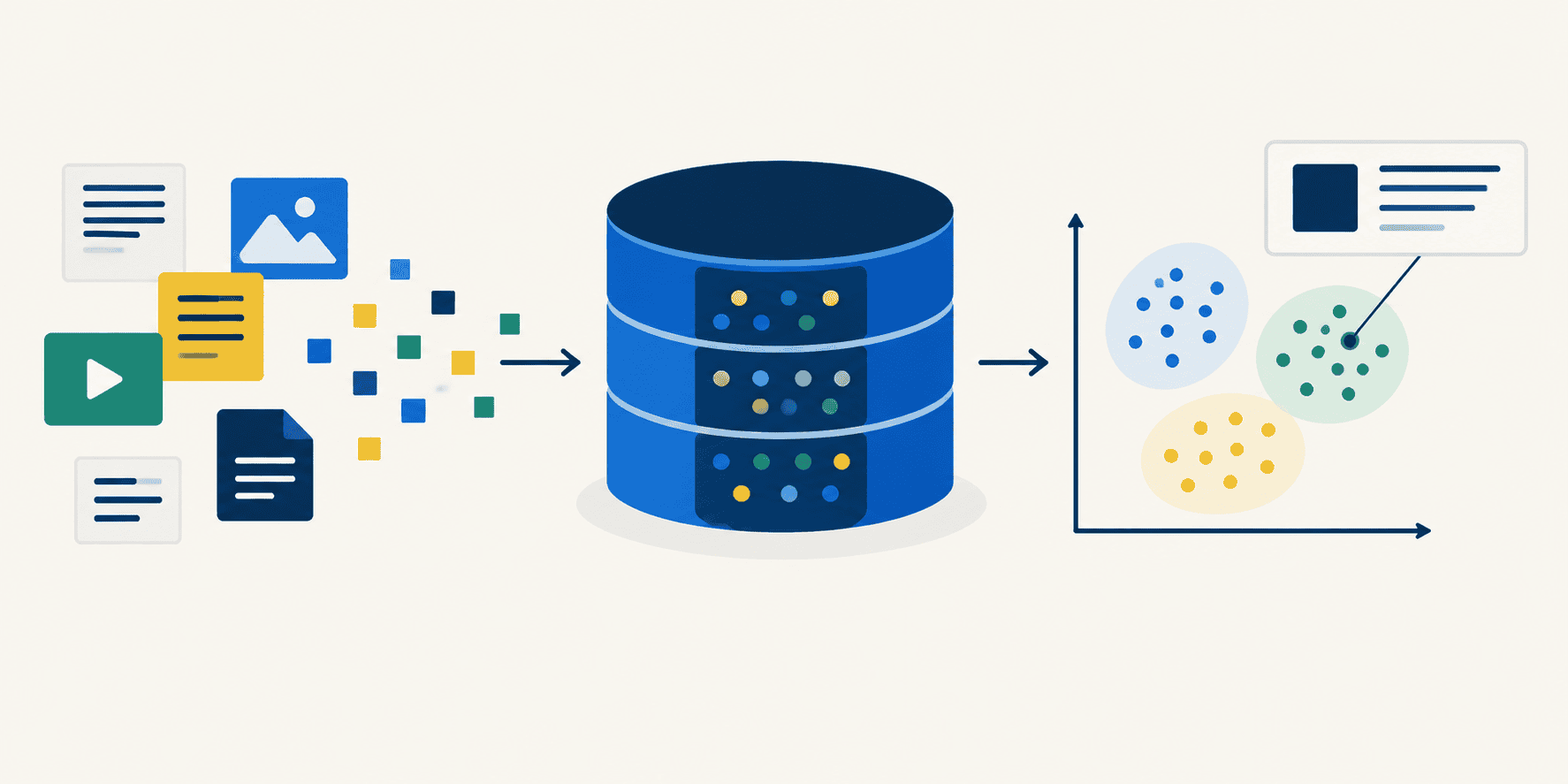
In this article, you will learn how a vector database works under the hood by building one from scratch in ten incremental steps using Python and NumPy. Topics we will cover include: How documents are encoded into fixed-size vectors and searched by meaning rather than by keyword. How to add metadata filtering, input validation, and persistence to a minimal vector database. How brute-force cosine similarity scales with corpus size, and when to consider approximate indexing. Introducing Vector Databases A vector database answers questions by meaning rather than by keyword. It operates by turning every document into a vector of numbers and then finding the numbers that point in a similar direction to your query (which has also been turned into a vector of numbers). This tutorial will demonstrate how to build a working vector database of your very own, through ten steps that each demonstrate one atomic idea. To follow along, create an empty script and name it something clever like tutorial.py. Append each step’s code to the script as you go and re-run it after you make sense of the commentary. The resulting output should make sense at that point. Nothing here needs a GPU or an API key; one small model downloads on the first run, and everything after that is plain NumPy. Step 1: Setup You need three files from this repository in your working directory: vector_db.py is the actual database which, yes, is already built for you… but the real magic is the understanding of the code and the interaction with it using the code herein. The good news is, once you go through this tutorial and understand the code, recreating the vector database on your own is nearly trivial. corpus.py contains 25 simulated sample documents and their topic tags. test.py is the test suite, only here to make you feel safe and secure that the vector database works properly as implemented, which you can verify by running at any point with python test.py. Install the two dependencies: pip install numpy sentence-transformers Now start your tutorial.py file with the imports and two small display helpers. show() prints a list of search results as score, topic, document (relied upon later). header() just labels each section so the growing script’s output stays readable. 1234567891011121314151617181920 import timefrom pathlib import Pathimport numpy as npfrom corpus import DOCS, METAfrom vector_db import VectorDBWIDTH = 64def header(title): print(f"\n{title}\n{'─' * len(title)}")def show(results): if not results: print(" (no matches)") for hit in results: text = hit.text if len(hit.text) 12} {'memory':>9} {'scan':>9} {'rank':>9}")for n in (1_000, 10_000, 100_000): rows = big[:n] scores = rows @ query_vector scan_ms = milliseconds(lambda: rows @ query_vector) rank_ms = milliseconds(lambda: np.argsort(scores)[::-1][:5]) print(f" {n:>12,} {rows.nbytes / 1024**2:>7.1f} MB " f"{scan_ms:>6.2f} ms {rank_ms:>6.2f} ms") Output: 10. How this scales────────────────── 14.9 ms per query over 25 documents documents memory scan rank 1,000 1.5 MB 0.01 ms 0.04 ms 10,000 14.6 MB 0.36 ms 0.55 ms 100,000 146.5 MB 3.73 ms 8.90 ms At 25 documents, embedding the query is essentially the entire computation, since the search itself is too fast to measure. Note that milliseconds() discards one warm-up run; the first call to a NumPy matrix routine spins up its internal thread pool, which can take more time than the actual work itself, with a result of making a small corpus look slower than a large one. Two things are worth pointing out in the results table above: Both columns grow linearly; nothing here is clever, it simply touches every row. Past ~100,000 rows the sort starts to outgrow the scan. At a million documents the scan takes about 25 ms and the full sort about 90 ms. That is the point where it pays to stop sorting everything (np.argpartition finds the top k in about 10 ms). Not far beyond this you will find the point where you reach for a real approximate index (HNSW, IVF) and trade a little accuracy for speed. Wrapping Up Every step here rests on a single idea: scale each embedding to length 1, and a plain dot product becomes cosine similarity. Ranking an entire corpus is then one matrix multiply. Everything else you added along the way — from metadata filters, saving and loading, the guard rails on add() — is bookkeeping that keeps documents, metadata and vectors in lockstep, so that the multiplication remains meaningful. The big takeaway — beyond the simplicity and elegance behind the implementation of a vector database’s core functionality — is that the design does not change between 25 documents and 25 million; only the index structure underneath it does. This is, not surprisingly, precisely what the managed vector databases are selling. For more information on vector databases from different points of view, check out these Machine Learning Mastery resources: Understanding RAG Part VII: Vector Databases & Indexing Strategies by Iván Palomares Carrascosa Vector Databases Explained in 3 Levels of Difficulty by Bala Priya C The Complete Guide to Vector Databases for Machine Learning by Bala Priya C No comments yet.